the Creative Commons Attribution 4.0 License.
the Creative Commons Attribution 4.0 License.
 | 07 Nov 2019
Description and evaluation of the tropospheric aerosol scheme in the European Centre for Medium-Range Weather Forecasts (ECMWF) Integrated Forecasting System (IFS-AER, cycle 45R1)
Zak Kipling
Johannes Flemming
Olivier Boucher
Pierre Nabat
Martine Michou
Alessio Bozzo
Melanie Ades
Vincent Huijnen
Angela Benedetti
Richard Engelen
Vincent-Henri Peuch
Jean-Jacques Morcrette
This article describes the IFS-AER aerosol module used operationally in the Integrated Forecasting System (IFS) cycle 45R1, operated by the European Centre for Medium-Range Weather Forecasts (ECMWF) in the framework of the Copernicus Atmospheric Monitoring Services (CAMS). We describe the different parameterizations for aerosol sources, sinks, and its chemical production in IFS-AER, as well as how the aerosols are integrated in the larger atmospheric composition forecasting system. The focus is on the entire 45R1 code base, including some components that are not used operationally, in which case this will be clearly specified. This paper is an update to the Morcrette et al. (2009) article that described aerosol forecasts at the ECMWF using cycle 32R2 of the IFS. Between cycles 32R2 and 45R1, a number of source and sink processes have been reviewed and/or added, notably increasing the complexity of IFS-AER. A greater integration with the tropospheric chemistry scheme of the IFS has been achieved for the sulfur cycle and for nitrate production. Two new species, nitrate and ammonium, have also been included in the forecasting system. Global budgets and aerosol optical depth (AOD) fields are shown, as is an evaluation of the simulated particulate matter (PM) and AOD against observations, showing an increase in skill from cycle 40R2, used in the CAMS interim ReAnalysis (CAMSiRA), to cycle 45R1.


Ambient air pollution is a major public health issue, with effects ranging from increased hospital admissions to increased risk of premature death. Globally, an estimated 4.2 million deaths are estimated to have been linked to outdoor air pollution in 2016 (World Health Organization report on ambient air quality and health, 2018; https://www.who.int/news-room/fact-sheets/detail/ambient-(outdoor)-air-quality-and-health, last access: 2 April 2019), mainly from heart disease, stroke, chronic obstructive pulmonary disease, lung cancer, and acute respiratory infections in children. A large part of this mortality rate is caused by exposure to small particulate matter of 2.5 µm or less in diameter (PM2.5), which is known to cause cardiovascular and respiratory disease, as well as cancer.
Aerosols also impact meteorological and climate processes and predictions, directly by scattering and absorbing incoming shortwave and longwave radiation through the aerosol–radiation interaction (ARI; Bellouin et al., 2005) and indirectly through aerosol–cloud interaction (ACI; Fan et al., 2016, for example). Most climate models represent the impact of aerosols (Bellouin et al., 2011b). Meteorological forecasts provided by the IFS have been shown to be improved through the use of more realistic aerosol climatologies (Rodwell and Jung, 2008; Bozzo et al., 2019). Mulcahy et al. (2014) corrected a significant bias in outgoing longwave radiative fluxes over the Sahara by including interactive aerosol direct and indirect effects in the Met Office Unified Model (MetUM).
Particles released by volcanic eruptions can also impact air traffic, as happened in April 2010 with the eruption of the Eyjafjallajökull volcano in Iceland, which led to a major disruption of European and transatlantic aviation. As a consequence, modelling and forecasting levels of particulate matter, with the highest possible level of accuracy, is a major concern of the public authorities worldwide and has been an important focus of the research community. In this context, the ECMWF is one of the first centres to propose operational global forecasts of aerosols. Besides the ECMWF, there are currently at least eight centres producing and disseminating near -real-time operational global aerosol forecasting products: the Japan Meteorological Agency (JMA), the NOAA National Centre for Environmental Prediction (NCEP), the US Navy Fleet Numerical Meteorology and Oceanography Centre (NREL/FNMOC), the NASA Global Modelling and Assimilation Office (GMAO), the UK Met Office, Météo-France, the Barcelona Supercomputing Center (BSC), and the Finnish Meteorological Institute (FMI). These groups are all members of the International Cooperative for Aerosol Prediction (ICAP; Sessions et al., 2015; Xian et al., 2019), which uses data provided by these centres in the ICAP Multi-Model Ensemble (ICAP-MME). The ICAP-MME dataset is updated daily and is available at https://www.usgodae.org/ftp/outgoing/nrl/ICAP-MME (last access: 2 September 2019). The World Meteorological Organization Sand and Dust Storm Warning Advisory and Assessment System (SDS-WAS; Terradellas, 2016) focuses on the prediction of dust aerosol and provides near-real-time analysis, forecasts, and evaluation at https://sds-was.aemet.es/ (last access: 2 September 2019). The ensemble prediction of aerosols is also a promising approach (Rubin et al., 2016). Numerous regional aerosol models have been developed; a detailed enumeration and description can be found in Kukkonen et al. (2011) and Baklanov et al. (2014).
The global monitoring and forecasting of aerosols is a key objective of the Copernicus Atmospheric Monitoring Service (CAMS), operated by the ECMWF on behalf of the European Commission. To achieve this, the ECMWF operates and develops the Integrated Forecasting System (IFS), which combines state-of-the-art meteorological and atmospheric composition modelling together with the data assimilation of satellite products in the framework of CAMS (2014 to present); before that the Monitoring Atmospheric Composition and Climate series of projects (MACC, MACC-II, and MACC-III; 2010 to 2014) and the Global and regional Earth-system Monitoring using Satellite and in situ data project were integrated (GEMS; 2005 to 2009; Hollingsworth et al., 2008). The MACC and CAMS projects are centred around operational near-real-time (NRT) forecasts and reanalyses of global atmospheric composition: the MACC reanalysis (Inness et al., 2013), the CAMS interim ReAnalysis (CAMSiRA; Flemming et al., 2017), and the CAMS reanalysis (CAMSRA; Inness et al., 2019). The IFS is originally a numerical weather prediction system dedicated to operational meteorological forecasts. It was extended to forecast and assimilate aerosols (Morcrette et al., 2009; Benedetti et al., 2009), greenhouse gases (Engelen et al., 2009; Agustí-Panareda et al., 2014), and reactive trace gases (Flemming et al., 2009, 2015; Huijnen et al., 2019). “IFS-AER” denotes the IFS extended with the bin–bulk aerosol scheme used to provide aerosol products in the CAMS project.
The atmospheric composition component IFS-AER was continually updated within the MACC and CAMS project, with yearly or twice yearly upgrades of the operational forecasting system that followed and included upgrades of the operational IFS. The code revisions that are integrated into the operational version of IFS-AER must satisfy the two conditions (one qualitative, one quantitative) that they bring the model closer to “physical” reality, i.e. that more processes and/or species are represented, and that they improve the skill scores against observations.
Besides its use in the CAMS project, different versions of IFS-AER have been adapted within the Météo-France CNRM climate model system (Michou et al., 2015); it is also part of the MarcoPolo–Panda ensemble dedicated to the forecast of air quality in eastern China (Brasseur et al., 2019), of which the ECMWF is a member.
Various versions of IFS-AER have been tested and used to improve meteorological forecasts by the ECMWF. This was done first by generating and implementing a 3-D aerosol climatology using IFS-AER (Bozzo et al., 2019). Interactive aerosols are also being experimented with in sub-seasonal forecasts with the IFS and were shown to have a significant and positive impact on the skill of these products because of an improved representation of the radiative impacts of dust and carbonaceous aerosols in particular (Benedetti and Vitart, 2018).
Morcrette et al. (2009), hereafter denoted as M09, and Benedetti et al. (2009) describe the aerosol modelling and data assimilation aspects, respectively, in cycle 32R2 of the IFS. This paper focuses on the updates in the forward model since 2009; the data assimilation aspects and the optical properties used are only briefly described.
The paper is organized as follows. Section 2 presents a general description of IFS-AER and how it is implemented in the IFS and interacts with other components of the forecasting system. Section 3 describes the model configuration used in the operational near-real-time (NRT) simulations. Section 4 focuses on the dynamical and prescribed aerosol emissions and production processes. Section 5 details the aerosol sink processes: dry and wet deposition and sedimentation. The aerosol optical properties and PM formulae are presented in Sect. 6. Section 7 presents simulation results and budgets; Sect. 8 is dedicated to a preliminary evaluation of simulations against aerosol optical depth (AOD) observations from the AERONET network (Holben et al., 1998) and against European and North American PM observations.
2.1 Atmospheric composition forecasts with the Integrated Forecasting System (IFS)
General aspects of the IFS and how they relate to atmospheric composition modelling are described in Flemming et al. (2015); a more detailed technical and scientific documentation of the cycle 45R1 release of the IFS can be found at https://www.ecmwf.int/en/forecasts/documentation-and-support/evolution-ifs/cycles/summary-cycle-45r1 (last access: 9 May 2019). The IFS is a numerical weather prediction (NWP) model operated by the ECMWF to provide operational weather forecasts with extensions to represent tropospheric aerosols, chemically interactive gases, and greenhouse gases. This integrated atmospheric composition forecasting system forms the core of the global system of the Copernicus Atmosphere Monitoring Service (CAMS); it is also used at a much higher resolution to provide operational meteorological forecasts. At the start of the time step, the three-dimensional advection of the tracer mass mixing ratios is simulated using a semi-Lagrangian (SL) method as described in Temperton et al. (2001) and Hortal (2002). Mass conservation of the transported tracers (aerosols and trace gases) can be an issue because the SL scheme is not formally mass conservative. Similarly to what is practised for trace gases (Flemming et al., 2015; Diamantakis and Flemming, 2014) and for greenhouse gases (Agusti-Panareda et al., 2017), a proportional mass fixer is used in order to ensure that the total global mass of aerosol tracers is conserved during advection. The aerosol tracers are mixed vertically by the turbulent diffusion scheme (Beljaars and Viterbo, 1998), which also simulates the injection of emissions at the surface and the application of the surface dry deposition flux as boundary conditions. The dry deposition velocity is estimated by IFS-AER depending on the land surface and meteorological conditions as outlined in Sect. 4. The aerosol tracers are further transported and mixed vertically by the shallow and deep convection fluxes (Bechtold et al., 2014). Since cycle 43R3, a new radiation package has been in use operationally in the IFS and is described in Hogan and Bozzo (2018). The shortwave and longwave aerosol–radiation interactions (ARIs) can be computed using an aerosol climatology based on the CAMS interim ReAnalysis (Bozzo et al., 2019). Optionally, the prognostic aerosol mass mixing ratio from IFS-AER can be used to dynamically compute the ARI; this option has been used in the operational context since cycle 45R1. The impact of using prognostic aerosols in the radiation scheme is generally small on simulated aerosol fields. There can occasionally be a large impact on surface temperature and on aerosol loading itself (e.g. Rémy et al., 2015) when the aerosol loading is particularly high. The use of interactive aerosols in the radiation scheme can also indirectly impact chemical species when running coupled with CB05, since photolysis rates are usually dependent on temperature. There is currently no representation of aerosol–cloud interactions (ACIs). Introducing a representation of ACI in IFS-AER is planned in the future. The aerosol tracers and related processes are represented only in grid-point space. The horizontal grid can be either a reduced Gaussian grid (Hortal and Simmons, 1991) or a cubic octahedral grid. The vertical distribution uses a hybrid sigma–pressure coordinate with 60 or 137 levels. In this paper, a horizontal spectral resolution of TL511 (equivalent to a grid box size of about 40 km) and a vertical resolution of 60 levels were used, which matches the resolution used operationally with cycle 45R1. The resolution used is much coarser than for the operational IFS operated by the ECMWF, which currently uses a TCO1279L137 resolution for its high-resolution simulations because of the numerical cost of the extra aerosol and trace gas (CB05) components. In an operational context there are tight constraints on time for the model to run, which effectively limits the horizontal and vertical resolution used with IFS-AER. The aerosol tracers in IFS-AER can either be initialized using the 4D-Var data assimilation of the IFS as described in Benedetti et al. (2009) or by the 3-D fields from the previous forecast (in so-called “cycling forecast mode”). In the latter case, the meteorological fields are provided by the ECMWF IFS operational analysis.
2.2 Atmospheric composition in the IFS
Tropospheric and stratospheric chemistry is represented in the IFS through the IFS-CB05-BASCOE system (Flemming et al., 2015; Huijnen et al., 2016). Tropospheric chemistry in the IFS is based on a modified version of Carbon Bond 05 (CB05; Yarwood et al., 2005), which represents 55 trace gases interacting through 93 gaseous, 3 heterogeneous, and 18 photolysis reactions. IFS-CB05 is described in detail in Flemming et al. (2015). Stratospheric chemistry is based on the Belgian Assimilation System for Chemical ObsErvations (BASCOE; Errera et al., 2008), which was first developed to assimilate satellite observations of stratospheric composition. The BASCOE version as adapted in the IFS includes 58 trace gases interacting through 142 gaseous, 9 heterogeneous, and 52 photolysis reactions. The merging of tropospheric and stratospheric chemistry parameterizations is described in detail in Huijnen et al. (2016). The representation of stratospheric chemistry through BASCOE is not used in the operational cycle 45R1. Alternative chemistry schemes, based on IFS-MOZART and IFS-MOCAGE, have also become available recently (Huijnen et al., 2019).
2.3 Main characteristics of IFS-AER
IFS-AER is a bulk–bin scheme derived from the LOA/LMDZ model (Boucher et al., 2002; Reddy et al., 2005) using mass mixing ratio as the prognostic variable of the aerosol tracers. The aerosol species and the assumed size distribution are shown in Table 1. The prognostic species are sea salt, desert dust, organic matter (OM), black carbon (BC), and sulfate and its gas-phase precursor, sulfur dioxide. IFS-AER can be run in stand-alone mode, i.e. without any interaction with the chemistry, or coupled with IFS-CB05. Sea salt is represented with three bins (radius bin limits at 80 % relative humidity are 0.03, 0.5, 5, and 20 µm). As described in Reddy et al. (2005), sea salt emissions as well as sea salt particle radii are expressed at 80 % relative humidity. This is different from all the other aerosol species in IFS-AER, which are expressed as dry mixing ratios (0 % relative humidity). Users should pay special attention to this when dealing with a diagnosed sea salt aerosol mass mixing ratio, which needs to be divided by a factor of 4.3 to convert to the dry mass mixing ratio in order to account for the hygroscopic growth and change in density. Desert dust is also represented with three bins (radius bin limits are 0.03, 0.55, 0.9, and 20 µm). For both dust and sea salt, there is no mass transfer between bins. Two components are considered of organic matter and black carbon: hydrophilic and hydrophobic fractions, with the ageing processes transferring mass from the hydrophobic to hydrophilic OM and BC. Sulfate aerosols and, when not fully coupled to IFS-CB05, its precursor gas sulfur dioxide are represented by two prognostic variables. When running fully coupled with IFS-CB05, which is not the operational configuration with cycle 45R1, sulfur dioxide is represented in CB05 and thus not in IFS-AER. For the optional nitrate species, two prognostic variables represent fine-mode nitrate produced by gas–particle partitioning and coarse-mode nitrate produced by heterogeneous reactions of dust and sea salt particles. In all, IFS-AER is thus composed of 12 prognostic variables when running stand-alone and 14 when fully coupled with IFS-CB05 (including nitrates and ammonium), which allows for a relatively limited consumption of computing resources, as shown in Table 2.
Table 1Aerosol species and parameters of the size distribution associated with each aerosol type in IFS-AER (rmod: mode radius, ρ: particle density, σ: geometric standard deviation). Values are for the dry aerosol apart from sea salt, which is given at 80 % relative humidity (RH).
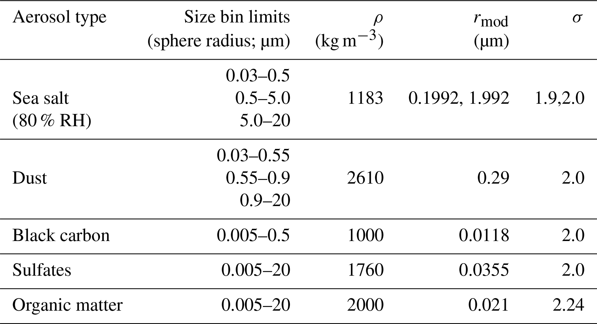
Table 2System Billing Unit (SBU) consumption of a 24 h forecast at TL511L60. SBU is a unit of CPU consumption used at the ECMWF; its precise definition can be found at https://confluence.ecmwf.int/display/UDOC/HPC+accounting (last access: 3 September 2019).

2.4 Coupling to the chemistry
IFS-AER can run coupled with the tropospheric chemistry scheme included in the IFS, CB05. The coupling is two-way and consists, on the chemistry side, of the use of aerosols in heterogeneous chemical reactions and the computation of the photolysis rates, which has been operational since cycle 43R3. On the aerosol side, the coupling is not used operationally and consists of the use of the gaseous precursors HNO3 and NH3 from IFS-CB05 for the production of nitrate and ammonium aerosols through gas partitioning and heterogeneous reactions on dust and sea salt particles, as described in Sect. 4. The updated concentrations of the precursor gases are passed back to IFS-CB05. Production rates of sulfate aerosols as estimated by IFS-CB05 can also be used in IFS-AER (this option is also not used operationally).
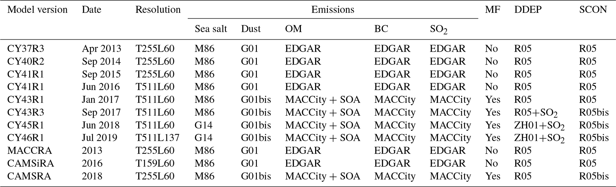
IFS-AER cycle 45R1 was operated by the ECMWF to provide operational near-real-time aerosol products in the framework of the Copernicus Atmospheric Monitoring Services until July 2019 when it was upgraded to cycle 46R1. The model is run in assimilation mode using AOD observations from MODIS collection 6 (Levy et al., 2013) and from the Polar Multi-Angle Product (Popp et al., 2016). Before cycle 45R1, only MODIS AOD was assimilated. IFS-AER cycles 36R1, 40R2, and 42R1 were used in assimilation to produce the MACC reanalysis (Inness et al., 2013), the CAMS interim ReAnalysis (Flemming et al., 2017), and the CAMS reanalysis (Inness et al., 2019). The operational configuration and the changes brought by successive cycles are presented at https://atmosphere.copernicus.eu/node/326 (last access: 2 September 2019). A summary of the operational configurations of the latest versions of the NRT system during the CAMS and MACC projects, as well as the three reanalyses, is shown in Table 3. The horizontal resolution was updated in June 2016, increasing from TL255 (approximately 80 km grid size) to TL511 (40 km). The vertical resolution increased from 60 to 137 levels in the upgrade to cycle 46R1 on 9 July 2019. Also, the CAMS reanalysis and the operational cycle 45R1 are run with interactive aerosols as an input of the radiative scheme to compute aerosol radiative interaction. The specific treatment of SO2 emissions over outgassing volcanoes was also introduced in cycle 45R1. The oceanic dimethylsulfide (DMS) source of sulfur dioxide was implemented in cycle 37R3 in April 2013. In the cycle 45R1 operational configuration, IFS-AER was run in stand-alone mode and not coupled with the chemistry. In the newly operational cycle 46R1, IFS-AER is now running coupled with the chemistry. A summary of the changes brought by the new cycle 46R1, not described in this article, can be found at https://atmosphere.copernicus.eu/node/472 (last access: 2 September 2019). Also, biomass burning injection heights are not used in the operational configuration of cycle 45R1 but are now used operationally in cycle 46R1.
Table 3IFS-AER cycles and options used operationally for near-real-time global CAMS products. MF stands for mass fixer, DDEP for dry deposition, and SCON for sulfate conversion. G01bis is for the Ginoux et al. (2001) dust emission scheme with a modified distribution of the emissions into the dust bins. R05bis is for the updated simple sulfate conversion scheme with temperature and relative humidity dependency. Cycle 46R1 also includes new developments not described in this article.
In IFS-AER, the sea salt and dust emissions are computed dynamically using prognostic variables from the meteorological model. The conversion of sulfur dioxide into sulfate aerosol and nitrate production also uses input from the meteorological model. The other aerosol species use external emissions datasets such as MACCity (Granier et al., 2011), CMIP6 (Gidden et al., 2019), or CAMS_GLOB. Aerosol emissions are released at the surface, except for emissions from biomass burning, which can optionally be released at an injection height, and SO2 emissions from outgassing volcanoes, which can optionally be released at the altitude of the volcano. In the operational 45R1 context, emissions from biomass burning are released at the surface, while SO2 emissions from outgassing volcanoes are released at the altitude of the volcano. Injection heights for biomass burning emissions are not used operationally in cycle 45R1 because their impact has not yet been sufficiently validated for trace gases: in an operational context it is important that biomass burning emissions of aerosols and trace gases are treated in the same way.
4.1 Organic matter and black carbon
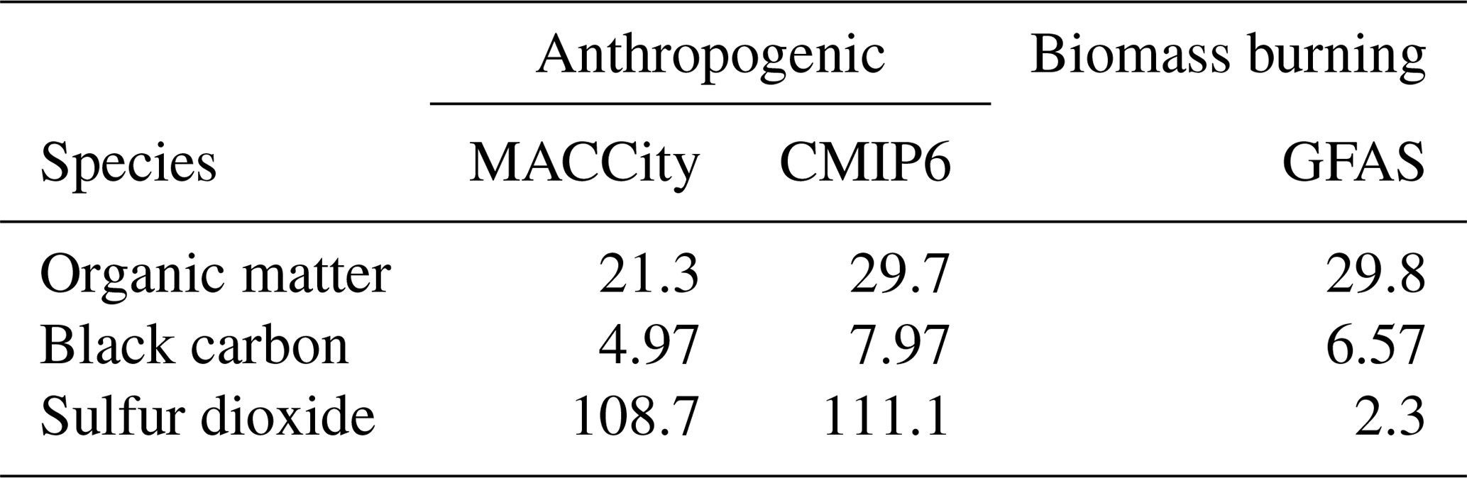
The anthropogenic (non-biomass burning) sources of OM and BC can be taken from the MACCity (Granier et al., 2011) or the more recent CMIP6 (Gidden et al., 2019) emissions datasets; for the operational cycle 45R1, analysis and forecast emissions from MACCity are used. These emissions inventories provide monthly emissions, updated from year to year for MACCity. MACCity emissions of black carbon are distributed by 20 % into the hydrophilic and the remaining 80 % into the hydrophobic black carbon tracers as in Reddy et al. (2005). MACCity emissions provide only organic carbon emissions rather than organic matter emissions. To translate these organic carbon emissions into OM emissions an OM:OC ratio of 1.8 is used. This is in the middle range of the OM:OC ratio provided by Canagaratna et al. (2015) and Philip et al. (2014). The OM emissions are then divided evenly between hydrophilic and hydrophobic OM. Table 4 reports the average yearly global anthropogenic emissions for the year 2014 from the three inventories. Biomass burning emissions from the Global Fire Assimilation System (GFAS) are also shown. The sulfur dioxide emissions are remarkably consistent between the two datasets. This is less the case for OM and BC.
Table 4Global emissions in 2014 of organic matter, black carbon, and sulfur dioxide (Tg yr−1). Anthropogenic (non-biomass burning) sources from MACCity and CMIP6 as well as biomass burning sources from GFAS are shown.
Biomass burning sources of OM and BC are provided by GFAS (Kaiser et al., 2012), which estimates these emissions (along with those of trace gases) using active fire products from the Moderate Resolution Imaging Spectroradiometer (MODIS) instrument onboard the Aqua and Terra satellites. Kaiser et al. (2012) compared cycling forecast simulations of biomass burning aerosols with simulations using data assimilation and concluded that a scaling factor of 3.4 should be applied to GFAS biomass burning sources when used in the IFS to minimize error compared to MODIS AOD. This means that the “perceived biomass burning emissions” of the model needed to fit observations are estimated based on GFAS data. The same method was used in Rémy et al. (2017) to derive distinct scaling factors for the OM and BC species, with scaling factors varying from 2.7 to 5 with an average of 3.2 for the former and from 4.9 to 7 with a 6.1 average for the latter. The use of scaling factors for biomass burning emissions is frequent; for example, a value of 1.7 is used in the Met Office Unified Model limited-area configuration over South America that was used for the South American Biomass Burning Analysis (SAMBBA) campaign (Kolusu et al., 2015), and values of 1.8 to 4.5 are used in GEOS-5 (Colarco, 2011). Some models such as CAM5 (Tosca et al., 2013) also use regional scaling factors (Lynch et al., 2016). The reasons why scaling factors are required are not fully elucidated. In the operational cycle, the 3.4 scaling factor of Kaiser et al. (2012) is used. Biomass burning emissions are by default released at the surface. This can be unrealistic: a large fraction of fires release smoke constituents in the planetary boundary layer (PBL), and a minority of very large fires emit large quantities of aerosols and trace gases in the free troposphere and even, for extreme cases, in the stratosphere (Fromm et al., 2005). The fraction of fires that emit aerosols and trace gases in the free troposphere was evaluated at 5 %–15 % by various authors (Kahn et al., 2008; Val Martin et al., 2010; Sofiev et al., 2012). The GFAS dataset also includes daily injection heights that are computed using two different methods: the IS4FIRE approach (Sofiev et al., 2013) and the Plume Rise Model (PRM; Freitas et al., 2010) approach. Injection heights from GFAS as estimated using the PRM can optionally be used for biomass burning emissions. Biomass burning aerosols are emitted at the mean height of maximum injection, which is defined as the average of the plume heights at which detrainment is above half the maximum value. The daily injection heights in GFAS are representative of the maximum value reached during daytime (see Rémy et al., 2017), so using these at night when the atmosphere is stable could lead to errors in the vertical distribution and transport of biomass burning aerosol plumes. To prevent this, injection heights are used only if the mean height of maximum injection is above 200 m and if the diagnosed PBL height is above 1500 m. Otherwise, the smoke constituents are released in the first three model levels above the surface.
Secondary organic aerosol (SOA) is formed from a variety of anthropogenic and biogenic gaseous and liquid precursors (Hallquist et al., 2009). A commonly used approach to represent these processes is the volatility basis set (VBS) scheme, used in GEOS-Chem (Jo et al., 2013; Hodzic et al., 2016) and in the ORACLE module of the EMAC model (Tsimpidi et al., 2014). A recent intercomparison (Tsigaridis et al., 2014) showed that most models underestimate the production of SOA. The treatment of secondary organic aerosol (SOA) is very simplistic in IFS-AER. SOA is treated as part of the organic matter species and is emitted at the surface. The biogenic component of SOA emissions is taken from the emissions inventory used for the 2006 AEROCOM model intercomparison exercise (Dentener et al., 2006), which estimates SOA emissions as a 15 % fraction of natural terpene emissions; biogenic SOA emissions stand at 19.1 Tg yr−1. Additionally and optionally, since cycle 43R1, the anthropogenic component of SOA production has been represented in a very simple way as a fraction of CO emissions from MACCity, following Spracklen et al. (2011). This option has been used operationally since cycle 43R1. Anthropogenic SOA emissions estimated using this method amount to 144 Tg yr−1, which is consistent with the estimate provided by Spracklen et al. (2011) and by Hodzic et al. (2016), for which best estimates of global SOA production stand at 132 Tg yr−1. Most speciated observations indicate that SOA is composed of a large fraction of surface aerosols, and this very simple representation helps in addressing a persistent underestimation of anthropogenic aerosols in the IFS. This new source of anthropogenic aerosols also had adverse impacts on PM simulations, leading to a large overestimation, especially over China (as noted in Brasseur et al., 2019). Work is ongoing to address this through establishing a coupling with precursor organic chemistry; as a temporary solution in the operational cycle 45R1, anthropogenic SOA emissions have been capped at 0.25 µg m−2 s−1. Figure 1 shows that the SOA emissions estimated with this method are concentrated in highly populated areas: China, India, Nigeria, Europe, and the eastern United States.
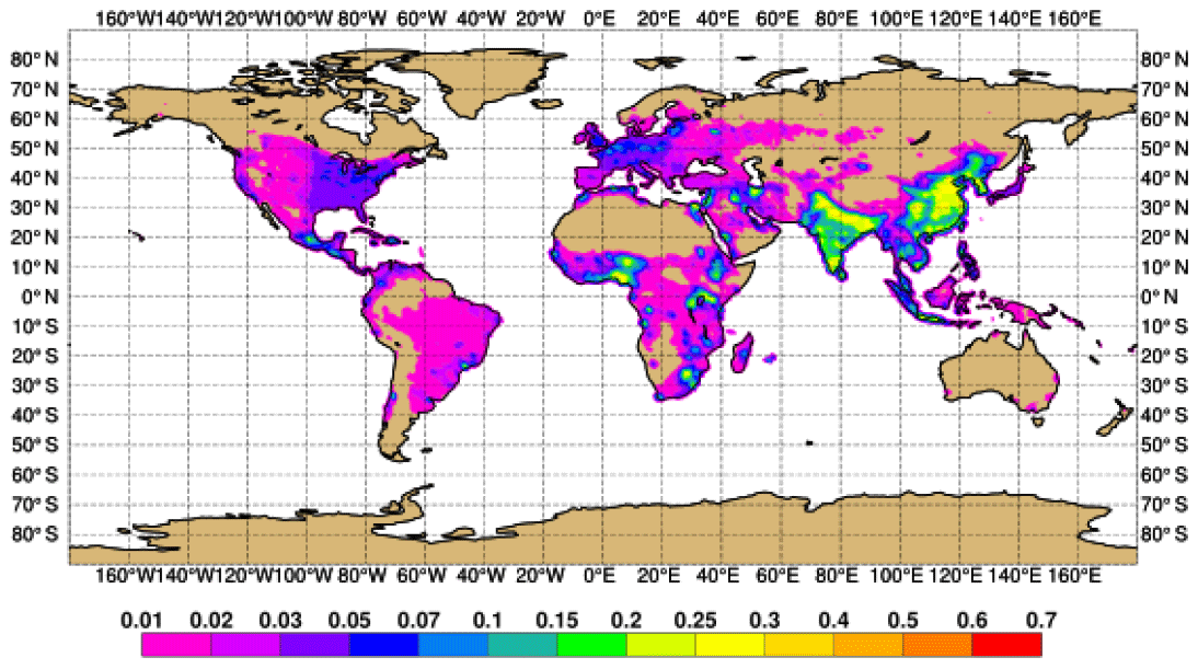
Figure 1Emissions of anthropogenic secondary organic aerosol (SOA) in 2017 (µg m−2 s−1), as used in cycle 45R1 of the IFS.
4.2 Sea salt
Sea salt is by far the most abundant aerosol species. In the IFS, two parameterizations of sea salt emissions are present: the Monahan et al. (1986) scheme, which was already present in cycle 32R2 and has been described in M09, and a new scheme following Grythe et al. (2014), which was implemented and became operational in cycle 45R1. The two schemes are denoted hereafter as M86 and G14, respectively.
The two schemes M86 and G14 both use mean wind speed as an input. Gustiness is accounted for in mean wind speed by adding a free convection velocity scale based on surface fluxes of sensible and latent heat to the horizontal velocity, following Beljaars and Viterbo (1998):
where U and V are the longitudinal and latitudinal wind speed at the lowest model level, zi is the PBL height, which is not a very critical input of this formula according to Beljaars and Viterbo (1998) and is taken as 1000 m in this expression, g is the gravitational constant, θv is the virtual potential temperature as defined in Stull (1988), and and are the surface fluxes of sensible and latent heat, respectively.
4.2.1 Monahan et al. (1986)
Monahan and Muircheartaigh (1980) suggested that the fraction of sea surface that is covered in white cap follows a wind speed dependency in the form of
From this, the production flux of sea salt aerosol is estimated by the following formula (Monahan et al., 1986):
where
and Dp is the particle diameter.
4.2.2 Grythe et al. (2014)
The more recent G14 parameterization has been implemented in the operational cycle 45R1. It combines emissions in different modes: 0.1, 3, and 30 µm dry diameter. A dependency of sea salt aerosol emissions on sea surface temperature following Jaeglé et al. (2011) is introduced, which increases emissions over the tropics and regions with warmer waters. This important increase in sea salt aerosol production with temperature is consistent with the conclusions of Sofiev et al. (2011) that modelled marine aerosol optical depth is generally too low in the tropics. Because of the scarcity and heterogeneity of the observational data there are large uncertainties in the temperature dependence of sea salt aerosol production (Grythe et al., 2014). The production of sea salt aerosol in G14 can be summarized as
where the sea surface temperature dependency factor is
Ocean salinity is not an input of the scheme, which is different from other schemes such as Sofiev et al. (2011). Ocean salinity varies a lot regionally, from 10 ‰ to 15 ‰ in the Baltic to more than 38 ‰ in the Mediterranean, for example. Cold-water tank experiments carried out by Zábori et al. (2012) indicated a dependency of sea salt aerosol production on salinity for salinity values up to 18 ‰. This means that overall the dependency of sea salt aerosol production on salinity can be considered weak, except regionally where salinity values are lower than 18 ‰.
Table 5 show the 2014 emissions (Tg yr−1) as estimated by the two schemes for the three sea salt bins. The total emissions of sea salt particles with a diameter below 10 µm are also shown to compare to other models as well as retrievals of emissions. The main difference between the two schemes concerns super-coarse sea salt, for which emissions are much higher with G14 compared to M86. This notably shifts the size distribution of sea salt at emission towards larger particles with G14. Grythe et al. (2014) provide a best estimate of global emissions derived from NOAA and EMEP PM10 observations of 10.2 Pg yr−1. Based on this, the G14 emissions are clearly closer to estimates.
Table 5Global emissions in 2014 (Pg yr−1) of fine, coarse, and super-coarse sea salt as estimated by the M86 and G14 schemes. The total emissions of particles with a diameter under 10 µm are also shown.
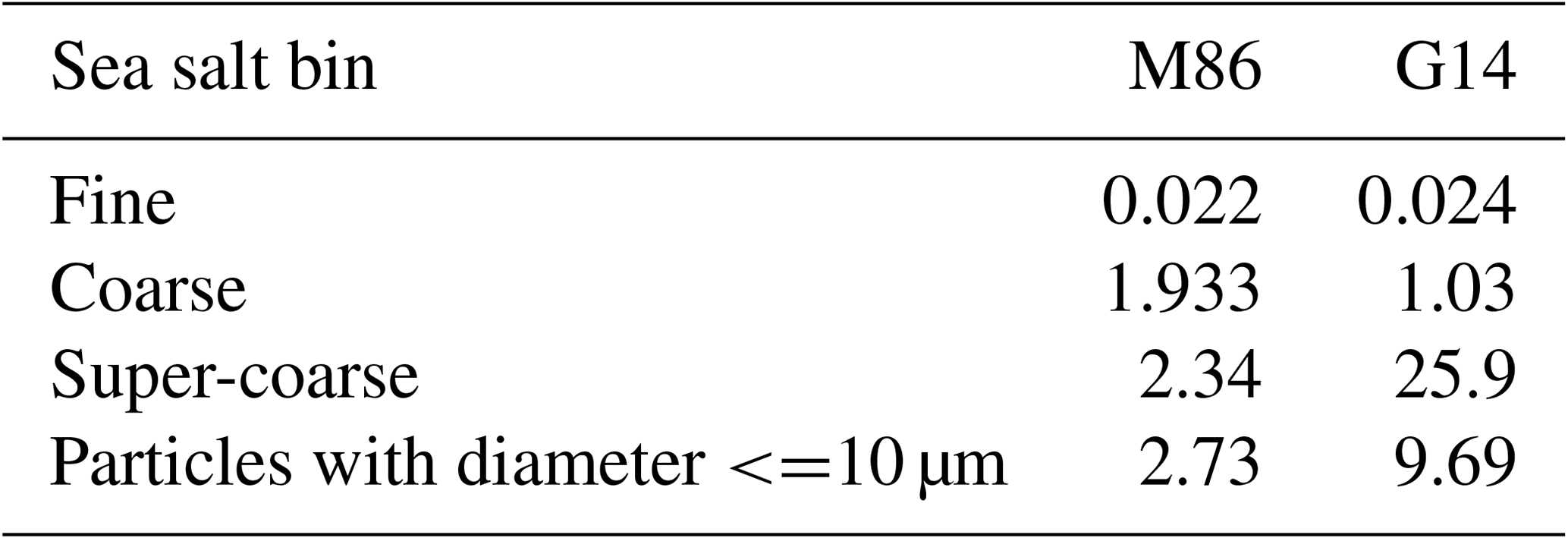
Figure 2 shows the 2017 emissions of super-coarse sea salt estimated by the two schemes. The annual production ranges from 0.005 to 0.02 kg m−2 yr−1 with M86. Production in the mid-latitudes with G14 is much higher than with M86, with values ranging from 0.1 to 0.4 kg m−2 yr−1. G14 stands out but more for the large increase in sea salt production in the tropics caused by the newly introduced dependency on sea surface temperature (SST). Production in the tropics ranges from 0.001 to 0.01 kg m−2 yr−1 for M86 and from 0.05 to 0.2 kg m−2 yr−1 for G14. It should be noted that over the Great Lakes area the production of sea salt aerosol is not zero for all schemes, which is clearly an artefact of the land–sea mask. This was corrected in later cycles.
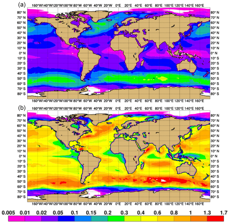
Figure 2The 2017 total emissions of sea salt aerosol at 80 % relative humidity from M86 (a) and G14 (b) (kg m−2 yr−1).
Figure 3 shows the bias in 2017 of total AOD simulated with cycle 45R1 IFS-AER using the M86 and G14 schemes as well as the observed and simulated AOD at the AERONET station of Ragged Point in the Antilles, which is one of the few stations that is mostly impacted by sea salt. The transatlantic transport of dust emitted in the Sahara also occasionally reaches the station. The G14 scheme increases simulated AOD to values that are generally closer to AERONET observations except in May–June and October–November. IFS-AER with M86 generally underestimates AOD over oceans. Compared to MODIS Aqua collection 6.1 AOD (Levy et al., 2013) at 550 nm, the global bias is reduced from −0.058 with M86 to −0.038 with G14. The 2017 average of daily root mean square error (RMSE) vs. MODIS AOD is slightly reduced from 0.083 to 0.08.

Figure 3The 2017 bias of simulated total AOD at 550 nm against MODIS Aqua collection 6.1 AOD; M86 (a) and G14 (b). (c) May–December 2016 daily AOD at 500 nm at the Ragged Point AERONET station, with observations from L2.0 AERONET (blue points), simulated by cycling forecast only IFS-AER using the M86 scheme (violet), and simulated by cycling forecast IFS-AER using the G14 scheme (black).
4.3 Dust
The parameterization of dust emissions has been left unchanged since M09. Only the distribution of dust emissions into the three dust bins has been modified. The formulation of Ginoux et al. (2001) is used. The areas likely to produce dust are first diagnosed using a combination of masks; potential dust-producing grid cells must satisfy the following criteria:
-
surface albedo is under 0.52;
-
the grid cell is entirely composed of land;
-
the snow cover is null;
-
the fraction of bare soil is above 0.1;
-
there is no ice and no wet skin;
-
the fraction of low vegetation is under 0.5;
-
there is no high vegetation; and
-
the standard deviation of subgrid orography is under 50 m.
For a potential dust-producing grid cell, the total dust flux is computed by
where Ut is the lifting threshold speed, S is a dust source function, and U10 gust represents the 3 s wind gusts computed using the mean wind including the gustiness effect U10 from Eq. (1) (Bechtold and Bidlot, 2009):
where z is the PBL height, taken as 1000 m here, u* is the surface friction velocity, and L is the Monin–Obukhov length scale defined as a function of surface fluxes of sensible and latent heat. This follows the parameterization of wind gusts in the IFS until cycle 33R1. The function f can be expressed as
Estimating the lifting threshold speed is a key part of any dust emission scheme; it depends on soil wetness, soil roughness, dust characteristics and mineralogy, and the size of the dust particles that are being lifted. In IFS-AER, a simple approach is used to estimate Ut:
where Ut0 and Dp0 are the “climatological” lifting threshold speed and dust particle radius at emission. The former varies between 3.5 m s−1 over the Taklimakan to 6 m s−1 over the Sahara, and the latter is set constant at 5 µm; w is the prognostic surface volumetric soil moisture. The lifting threshold speed is similar for each dust bin and is shown in Fig. 4. Values are highest over the Sahara, above 5 m s−1, while areas of very low values (0.1–1 m s−1) can be found in some boreal regions. The relatively low values over the Taklimakan and Gobi can explain the high dust emissions over these regions. The dust source function S is proportional to surface albedo. Equation (8) provides an estimate of the total emitted dust flux, which has to be distributed into the three dust bins. Until cycle 43R1, the distribution was 8 % of emissions into fine dust, 31 % into coarse dust, and 61 % into super-coarse dust. Comparing these values to the observed size distribution of dust aerosols at emission provided by Kok (2011) showed that the relative fraction of super-coarse particles was too low and the relative fraction of fine particles too high. In the CAMS reanalysis (Inness et al., 2019) and in the operational cycles from 43R1 onward, the distribution of total emissions into the dust bins was revised as follows: 5 % into fine dust, 12 % into coarse dust, and 83 % into super-coarse dust. Even though the total emissions are left unchanged, this change in distribution led to a significant decrease in the simulated burden and AOD of dust aerosols because the lifetime of super-coarse dust is shorter than for the other two bins as it is subject to a large sedimentation rate. Figure 5 shows the 2017 emissions of total dust, i.e. the sum of the three bins. The highest emissions, at 0.2–0.3 kg m−1 yr−1, occur in the Gobi and Taklimakan, which were impacted by severe dust storms in particular in May 2017. The Sahara, the Arabian Peninsula, and parts of Iran and Turkestan are also prominent. The emissions are very widespread in these regions, which is probably not realistic. Maps of the frequency of occurrence of dust AOD as retrieved using MODIS deep blue information (see Ginoux et al., 2012, for more details on the method) exceeding different thresholds can also serve as dust source functions. These show much higher maxima and lower minima in the Sahara and Arabian Peninsula, which confirms that the current operational approach could be refined.
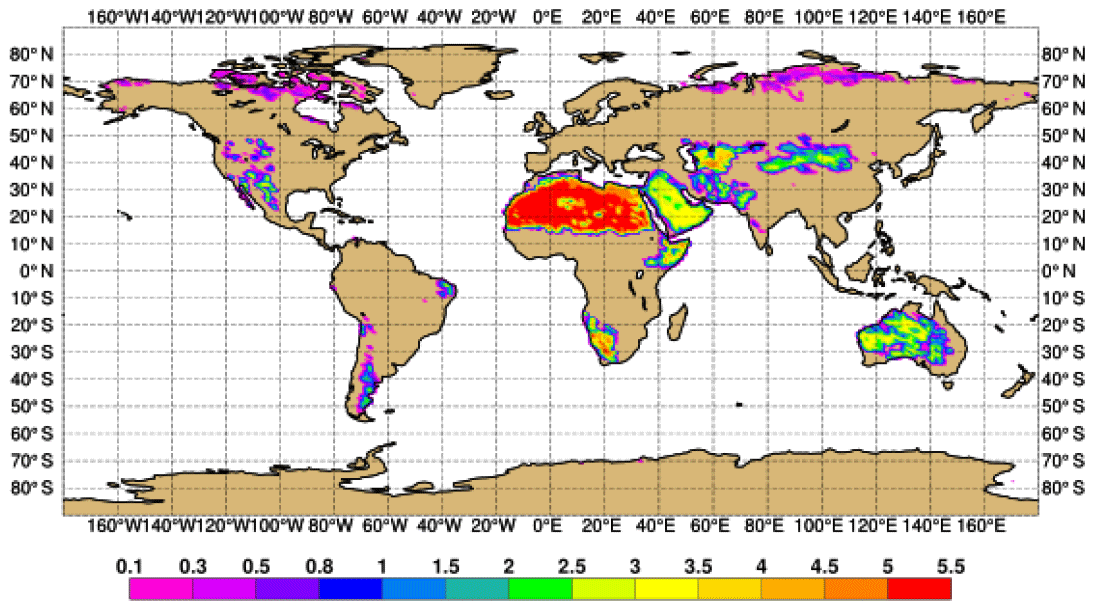
Figure 4The 2017 lifting threshold speed (m s−1).

Figure 5The 2017 total emissions of dust aerosol (kg m−2 yr−1).
4.4 Sulfur dioxide and sulfate
When running stand-alone (i.e. without the chemistry), sulfur dioxide is included in the tracers of IFS-AER; when running coupled with chemistry, sulfur dioxide is a prognostic species of the chemistry scheme, and oxidation rates provided by IFS-CB05 are used instead. Here we describe emissions and sources of sulfur dioxide in the stand-alone case. Similarly to OM and BC, emissions from MACCity, CMIP6, and other inventories can be used; the global averages are shown in Table 1. The emissions are the same as used in IFS-CB05. Optionally, these anthropogenic sources can be divided into “low sources”, which take 20 % of anthropogenic emissions, and “high sources”, which take the remaining 80 %. If this option is activated, then high sources are released in the first four model levels, whereas low sources are released at the surface. This option was not used in operational forecasts except in the CAMS reanalysis. A known issue of the CAMS reanalysis is an amount of sulfate aerosols that is too high above outgassing volcanoes, such as Kilauea in Hawaii and Popocatépetl in Mexico (Inness et al., 2019). To prevent this, emissions of sulfur dioxide above volcanoes can optionally be distinguished from the general case: if sulfur dioxide emissions occur above a volcano, then the emissions are distributed between the four model levels that are above the real altitude of the volcano instead of being emitted at the surface. Biomass burning sources of sulfur dioxide are provided by GFAS. In cycle 38R2 a source of sulfur dioxide from oceanic dimethylsulfide (DMS) was introduced. This new source is parameterized following Liss and Merlivat (1986):
where [DMS] is the concentration of DMS at the surface of the ocean (nmol L−1), as provided by an ancillary file, is the molar mass of sulfur dioxide, and Zl is a transfer speed computed as a function of wind speed, sea surface temperature, and sea ice fraction following Curran and Jones (2000).
Si is the sea ice fraction and Sc is the dimensionless Schmidt number, which is used to characterize flows in which viscosity and mass transfer are involved. Sc is computed as a function of ocean skin temperature in degrees Celsius Tsk:
In all, the source of sulfur dioxide from oceanic DMS stands at 30 Tg yr−1 on average.
The conversion of sulfur dioxide into particulate sulfate is treated in a very simple way following Huneeus (2007). In cycles 43R1 and before, conversion was parameterized only as a function of latitude as a proxy for the abundance of the OH radical. The conversion rate (per second) can be written as
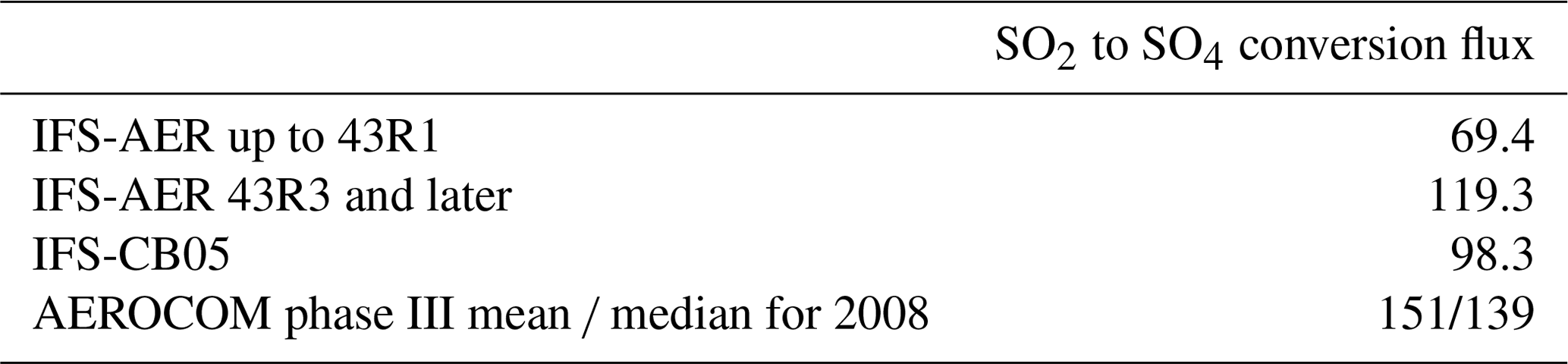
where δt is the time step, θ is the angular latitude, and C1 and C2 are e-folding times in days representing the lifetime at the pole and the Equator set to 8 and 5 d, respectively, for operational cycles up to 43R1. For the CAMS reanalysis and for operational cycles 43R3 and later, the values of C1 and C2 were set to 4 and 3.5 d, respectively, leading to higher production over most of the globe. This modification, together with the implementation of the dry deposition of SO2, was meant to shorten the lifetime of sulfate and reduce its burden, which was much too high in CAMSiRA as detailed in Flemming et al. (2015). These changes were successful in significantly reducing the burden of sulfate in the later CAMSRA (Inness et al., 2019). For the CAMS reanalysis and in operational cycles 43R3 and after, a diurnal cycle and a simple dependency on temperature following Eatough et al. (1994) and on relative humidity were introduced, and the new conversion rate is expressed as
where D(lt) is a cosine diurnal cycle function of local time, with a maximum value of 2 at midday local time and a minimum value of 0 at midnight local time. IRH is an increment factor set to 2 when RH is above or equal to 98 % and set to 1 otherwise. The difference arises from the fact that where RH is above 98 % the grid cell is supposed to be at least partly saturated, which leads to more active conversion from sulfur dioxide to sulfate aerosol. As shown in Table 6, these modifications led to a significant increase in the conversion of sulfur dioxide into particulate sulfate. Sulfur oxidation rates provided by IFS-CB05, which are used when IFS-AER is run coupled with the chemistry, are also shown and stand between the older and newer value using the conversion scheme of IFS-AER. The mean and median of the conversion process from AEROCOM phase III (Bian et al., 2017) are also shown for the year 2008. Accounting for the fact that sulfur dioxide emissions were higher in 2008 than in 2014 by around 7 % in the MACCity inventory, the value for IFS-AER cycles 43R3 and later is quite close to the AEROCOM median. The changes in the sulfate conversion implemented for the CAMS reanalysis and in the operational cycles 43R3 and beyond (conversion constants, temperature, and relative humidity dependency) are meant to help address the problem of a sulfate burden that is too high in the CAMS interim ReAnalysis (Flemming et al., 2017) and also in the operational NRT runs before cycle 43R3. They are meant to reduce the concentrations of sulfate in the middle and upper troposphere and shorten the lifetime of both sulfate and sulfur dioxide. With a faster life cycle and reduced concentrations above the planetary boundary layer, the fraction of the mass mixing ratio increments distributed to sulfate during the data assimilation stage has been generally reduced in the CAMS reanalysis and in cycle 43R3 and beyond, leading to an important decrease in the total burden of sulfate in the CAMS reanalysis compared to the CAMS interim ReAnalysis, as well as in the operational cycles 43R3 and beyond.
Table 6Global conversion of sulfur dioxide into particulate sulfate in 2014 (Tg SO4 yr−1).
4.5 Nitrate and ammonium
With the important decrease in anthropogenic emissions of sulfur dioxide in recent years, the relative importance of nitrate and ammonium has increased (Bellouin et al., 2011b). The production of nitrate and ammonium aerosols in IFS-AER when running coupled with IFS-CB05 was introduced in cycle 45R1 but is not used operationally. The parameterization of the production of fine-mode nitrate and ammonium from gas-to-particle partitioning and of coarse-mode nitrate from heterogeneous reactions over dust and sea salt particles follows the approach of Hauglustaine et al. (2014), which is summarized below. The precursor gases HNO3 and NH3 are prognostic variables of IFS-CB05; their treatment is described in Flemming et al. (2015), while SO2 and HNO3 are evaluated in Huijnen et al. (2019).
4.5.1 Gas-to-particle partitioning
The most abundant acids in the troposphere are sulfuric acid (H2SO4) and nitric acid (HNO3). NH3 acts as the main neutralizing agent for these two species. As a first step, ammonium sulfate is formed from H2SO4 and NH3, only limited by the less abundant of the two species. This reaction takes priority over the formation of ammonium nitrate (NH4NO3) because of the low vapour pressure of sulfuric acid. The main reaction pathways are as follows.
Following Metzger et al. (2002), depending on the relative concentrations of ammonia and sulfate, three domains are considered to characterize how ammonium sulfate is formed. The total ammonia, sulfate, and nitrate concentrations are defined as follows.
For ammonia-rich conditions (TA>2TS) Reaction (3) is considered; for sulfate-rich conditions ( and TA>TS) Reaction (2) is considered, and finally for very sulfate-rich conditions () Reaction (1) is considered. As a second step, if NH3 is still present after Reactions (1), (2), or (3) then it is used for the neutralization of HNO3 by the following reaction.
The equilibrium constant Kp of Reaction (4) depends strongly on relative humidity and temperature. The parameterization of Mozurkewich (1993) is used to represent this dependence. Total ammonia that remains after Reactions (1), (2), or (3) is written as
where the value of Γ is 1, 1.5, or 2 depending on whether Reactions (1), (2), or (3) took place, respectively. If then ammonium nitrate is formed and its concentration is calculated by
Otherwise, ammonium nitrate dissociates and
Reaction (5) also allows us to compute the concentration of NH3 at equilibrium; the concentration of particulate NH4 is then given by
Finally, the updated concentrations of the precursor gases, [NH3] and [HNO3], are passed back to IFS-CB05.
4.5.2 Heterogeneous production
Gaseous HNO3 can also condense on large particles. The formation of smaller nitrate and ammonium particles through gas-to-particle partitioning is solved first because the equilibrium is reached faster (Hauglustaine et al., 2014). After the smaller particles are in equilibrium, the condensation of HNO3 on larger particles is treated. Heterogeneous reactions of HNO3 with calcite (a component of dust aerosol) and sea salt particles are accounted for through the following reactions.
While the NaCl species is similar to sea salt aerosols, calcite (CaCO3) is one of the many components of dust aerosol. In Fairlie et al. (2010) and Hauglustaine et al. (2014), the concentration of calcite is taken as 3 or 5 % of the total concentration of dust aerosol. An experimental version of IFS-AER that simulates a simplified dust mineralogy was used to compute a climatology of airborne calcite using as an input the dataset of Journet et al. (2014), which provides an estimate of the calcite content in the clay and silt fraction of soils. Figure 6 shows the vertically integrated fraction of airborne calcite in coarse and super-coarse dust. The regional differences are great, especially for calcite emitted from clay surfaces compared to coarse dust.
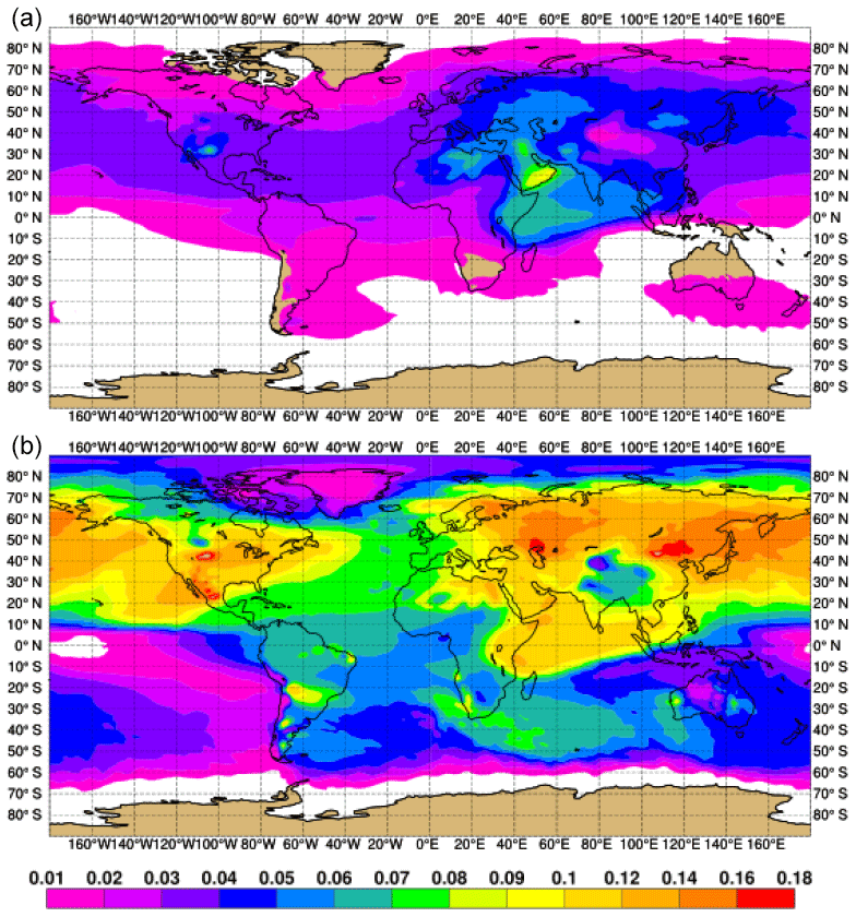
Figure 6Average fraction of calcite over super-coarse (a) and coarse (b) dust.
A 1st-order update parameterization is used to represent the uptake of HNO3 over sea salt and calcite particles. The rate constants of Reactions (8) and (9) are computed in a simplified way compared to the original scheme of Hauglustaine et al. (2014) for each sea salt (SS) and desert dust (DD) bin i:
where DSSi is the mass median diameter of sea salt bin i, DDDi is the mass median diameter of desert dust bin i, and NSSi and NDDi are the number concentration for the sea salt and desert dust bin i, respectively, computed using the mass concentration and the mass median diameter. Dg is the pressure- and temperature-dependent estimated molecular diffusion coefficient, ν is the temperature-dependent estimated mean molecular speed, and γ is the reactive uptake coefficient. For sea salt, as in Fairlie et al. (2010), a dependence of the uptake coefficient on relative humidity is used. Similarly to the gas-to-particle partitioning reactions, the updated concentration of HNO3 is passed back to IFS-CB05. The concentrations of the desert dust and sea salt bins are also updated depending on the amount of coarse-mode nitrate that is produced.
The production rate of fine-mode nitrate in 2014 is estimated at 2.16 Tg N yr−1, which is significantly below the 3.24 Tg N yr−1 for the year 2000 reported in Hauglustaine et al. (2014). For coarse-mode nitrate, 12.36 Tg N yr−1 was produced, which is higher than the 11.16 Tg N yr−1 reported in Hauglustaine et al. (2014). In both cases, different concentrations of the precursor gases as well as dust and sea salt aerosols are a large source of differences between the original implementation and the adaptation in IFS-AER. Figure 7 shows the 2014 average of fine-mode and coarse-mode nitrate and ammonium mass mixing ratios. Higher fine-mode nitrate surface concentrations are collocated with heavily populated areas and regions with high agricultural activity, reaching 3 to 5 µg m−3 over Europe and the US and up to 9–12 µg m−3 over parts of India and China. Coarse-mode nitrate is produced primarily over oceans close to heavily populated areas such as the eastern and western extremities of the Atlantic and Pacific oceans. Ammonium surface concentrations show similar patterns as fine-mode nitrate, with values between 1 and 2 µg m−3 over Europe, slightly less over the US, and 3 to 4 µg m−3 over the heavily populated parts of India and China.
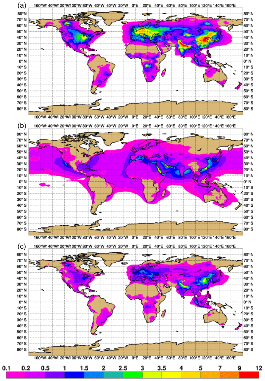
Figure 7The 2014 average of surface fine-mode and (a) coarse-mode (b) nitrate mass concentration and ammonium (c) surface concentration (µg m−3).
4.6 Ageing and hygroscopic growth
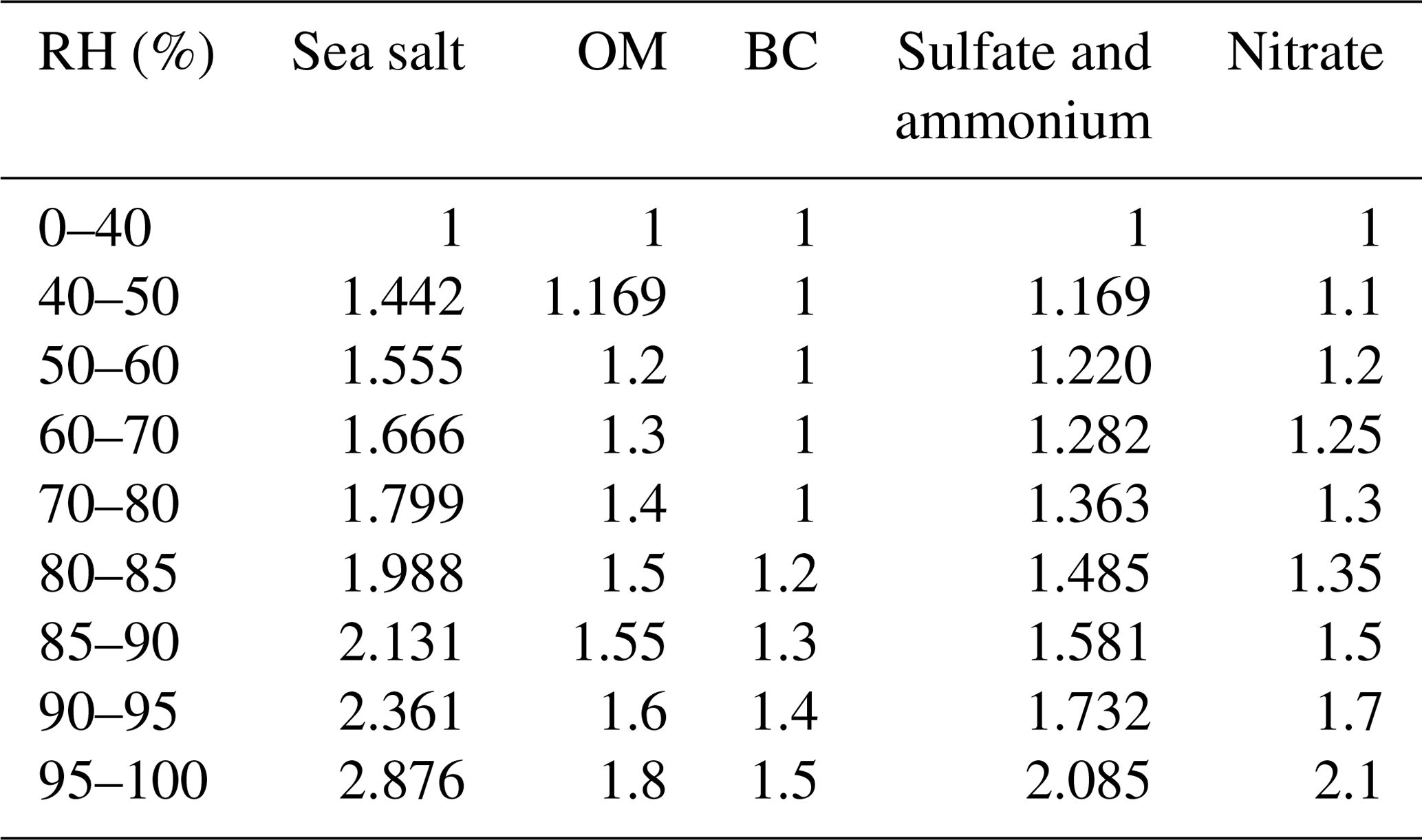
Hygroscopic growth is the process whereby, for some aerosol species, water is mixed in the aerosol particle, increasing its mass and size and decreasing its density. This process is treated implicitly in IFS-AER, since size is not resolved. It plays an important role, however, in the computation of optical properties and also for sinks that are size and/or density dependent, in particular dry deposition. The species subjected to hygroscopic growth in IFS-AER are sea salt, the hydrophilic components of OM and BC, sulfate, nitrate, and ammonium. The amount of water that is mixed in the aerosol particle depends on particle size. Table 7 details the changes in size for the concerned species. The values are drawn from Tang and Munkelwitz (1994) for sea salt, Tang et al. (1997) for sulfate and ammonium, Chin et al. (2002) for BC, and Svenningsson et al. (2006) for nitrate. For OM, the values are derived from the water-soluble organic (WASO) component of the OPAC (Optical Properties of Aerosols and Clouds) database (Hess et al., 1998).
For OM and BC, once emitted, the hydrophobic component is transformed into a hydrophilic one with an exponential lifetime of 1.16 d, shorter than in Reddy et al. (2005) wherein the lifetime is 1.63 d. This is closer to more recent measurements of black carbon ageing, which range from 8 to 23 h over Beijing and Houston, respectively (Wang et al., 2018).
Table 7Hygroscopic growth factor depending on ambient relative humidity.
Removal processes consist of dry and wet deposition and sedimentation or gravitational settling. Wet deposition and sedimentation are similar to M09, but they are described again here for completeness.
5.1 Dry deposition
Two schemes to compute the dry deposition velocities coexist in IFS-AER: the scheme from Reddy et al. (2005) or R05 used in the CAMS reanalysis and in operational cycles up to 43R3 and the newly implemented Zhang et al. (2001) or ZH01 scheme that computes the dry deposition velocities online. Until the operational cycle 45R1, the dry deposition velocity was used to directly compute a dry deposition flux:
where C is the aerosol mass mixing ratio at the lowest model level, ρ is the air density, and VDD is the dry deposition velocity. Since the operational cycle 45R1, the dry deposition velocity has been passed through to the vertical diffusion scheme, which directly updates the surface concentration at the lowest level. Before cycle 45R1, the dry deposition flux was instead added to the surface flux. The difference between the two approaches has been evaluated and found to be extremely small. Also, since cycle 43R3, the dry deposition of sulfur dioxide has been represented and is described below.
5.1.1 R05 dry deposition velocities
In the R05 scheme, dry deposition velocities are fixed for each aerosol tracer over continents and oceans. The values used in IFS-AER are shown in Table 8: the values over oceans and land differ only for sea salt and sulfate aerosols. Since operational cycle 45R1, a cosine function of local time has been applied as a diurnal cycle modulation of the fixed velocities, with a maximum of 1.7 at midday local time and a minimum of 0.3 at midnight. This is to account for the fact that dry deposition velocities display a marked diurnal cycle (Zhang et al., 2003) because of lower aerodynamic and canopy resistance. Also, over ice and snow surfaces, dry deposition velocities cannot exceed 0.3 mm s−1.

5.1.2 ZH01 dry deposition velocities
The ZH01 scheme is itself based on the dry deposition model of Slinn (1982). The deposition velocity at the surface is evaluated for all aerosol prognostic variables as
Compared to the original implementation of this scheme in Zhang et al. (2001), gravitational settling is not included in this equation as it is taken care of in another routine. Ar is the aerodynamic resistance, independent of the particle type, computed by
where k is the von Kármán constant, z0 is the roughness length provided by the IFS, z the height of the first model level, and u* the surface friction velocity. Sr in Eq. (21) is the surface resistance:
where EB, EIM, and EIN are the collection efficiencies for Brownian diffusion, impaction, and interception, respectively.
where Sc is the particle Schmidt number computed by ; ν is the kinematic viscosity of air, D is the particle diffusion coefficient, and YR is a surface-dependent constant with values provided in Table 3 of Zhang et al. (2001).
where St is the Stokes number for a smooth and rough flow regime.
where Dvisc is the dynamic viscosity of air, computed as a function of temperature only, and Vg is the gravitational velocity computed as
CF is the Cunningham slip correction to account for the viscosity dependency on air pressure and temperature; ρ and Dp are the particle density and diameter, respectively. For Dp, the mass median diameter (MMD) of each aerosol prognostic variable is used, and hygroscopic growth is taken into account for the relevant species. The Cunningham slip correction is defined differently from the original Zhang et al. (2001) implementation:
where λ is the mean free path of air molecules, and σ is the standard deviation of the assumed log-normal distribution of the considered particle. The impact of the different formulation of CF has been shown to be extremely small; α and CR are surface-dependent constants, whose values are provided in Table 3 of ZH01. Finally,
The IFS surface model distinguishes nine surface classes, which are given as fractions (tiles) for each grid box. The two vegetation tiles (“high” and “low” vegetation) are further classified according to 20 vegetation tiles. For the low and high vegetation tiles the IFS vegetation types were mapped to the 15 land classes of the ZH01 surface classes. The dry deposition velocity computed with this algorithm is computed three times for the three dominant tile fractions of each grid cell if they are defined, which gives a component of subgrid variability to the ZH01 scheme as it is implemented in IFS-AER. The final dry deposition velocity is the average of these three dry deposition velocities weighted by the relative fraction of the three dominant tile fractions. As shown in Khan and Perlinger (2017), the ZH01 parameterization's most sensitive input is particle size. Dry deposition velocities computed with the ZH01 algorithm decrease with particle diameter for diameters between 0.001 and 1 µm and increase for diameters between 1 and 10 µm.
Table 9 provides a comparison of the global dry deposition velocities in 2014 computed with the R05 and ZH01 methods. Values are on average generally lower with ZH01 compared to R05 for fine particles except for fine-mode dust. For super-coarse particles, on the other hand, values estimated with ZH01 are on average higher. Figure 8 shows monthly averages of the dry deposition velocities of super-coarse sea salt for January and July 2014. Values with R05 differ only for regions where snow or sea ice is present because of the 3 mm s−1 threshold over these areas. Elsewhere, values are very close between oceans and continents as the prescribed value is very close for both surfaces: 1.2 and 1.5 cm s−1, respectively. Values with ZH01 also show this dichotomy between regions free of ice and snow and the rest; however, the dry deposition velocities also vary a lot more elsewhere, with generally higher values over continents than over oceans because of rougher surfaces. This is more marked for the dry deposition velocities of super-coarse sea salt or dust, for which values over continents are 2 to 4 times larger than over oceans.
Table 9The 2014 global average of dry deposition velocities computed with R05 and ZH01 (m s−1).

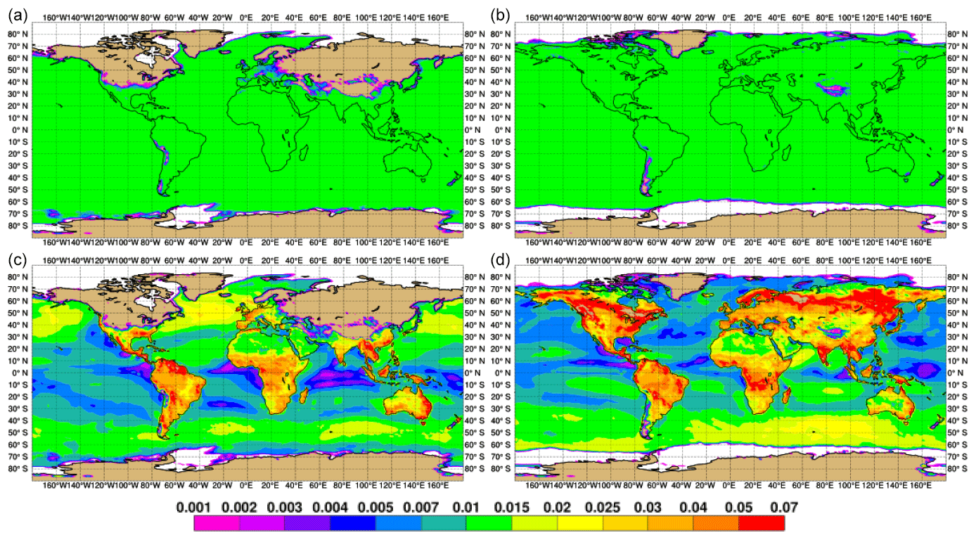
Figure 8January (a, c) and July (b, d) 2014 average of the dry deposition velocity of super-coarse sea salt computed with R05 (a, b) and ZH01 (c, d) (m s−1).
The impact of using the ZH01 or the R05 dry deposition schemes is important for simulations of aerosol optical depth and even more so for simulations of surface concentrations and PM. There are still some issues with the ZH01, notably dry deposition velocity and flux values that are too high over mountainous terrain. This particular problem has been addressed in cycle 46R1 of IFS-AER.
5.1.3 Dry deposition of sulfur dioxide
Dry deposition is an important sink for gaseous sulfur dioxide. For IFS-AER in stand-alone mode, this process has been represented since cycle 43R3 and is represented in the CAMS reanalysis. The approach is different from the other aerosol tracers and is similar to what is done for sulfur dioxide in IFS-CB05. Monthly sulfur dioxide dry deposition velocities have been computed offline using the approach described in Michou et al. (2004). These dry deposition velocities are applied to the sulfur dioxide tracer in IFS-AER, modulated by the same diurnal cycle as used for the R05 dry deposition velocities. The dry deposition of sulfur dioxide in 2017 was estimated at 51 Tg yr−1 compared with 138 Tg yr−1 of sulfur dioxide emissions.
5.2 Sedimentation
Sedimentation was also left broadly unchanged compared to M09. It is applied only for super-coarse dust and sea salt, for which it is an important sink. The change in mass mixing ratio from sedimentation follows the approach of Tompkins (2005) for ice sedimentation. The change in mass concentration caused by a transport in flux form at velocity Vs is given by
where ρ is the air density. The integration of this gives for each level k and time step j
which is solved from top to bottom. The gravitational velocity Vs is horizontally and vertically invariant for the two sedimented species and is computed using Stokes' law:
where ρp is the particle density, g the gravitational constant, μ the air viscosity, and CF the Cunningham correction factor.
5.3 Wet deposition
Wet deposition has been modified very little compared to M09. All aerosol tracers are subjected to wet deposition except hydrophobic OM and BC as well as sulfur dioxide. Both in-cloud (or rainout) and below-cloud (or washout) processes are represented.
5.3.1 In-cloud wet deposition (rainout)
The in-cloud scavenging rate (s−1) at model level k of an aerosol i is written as follows:
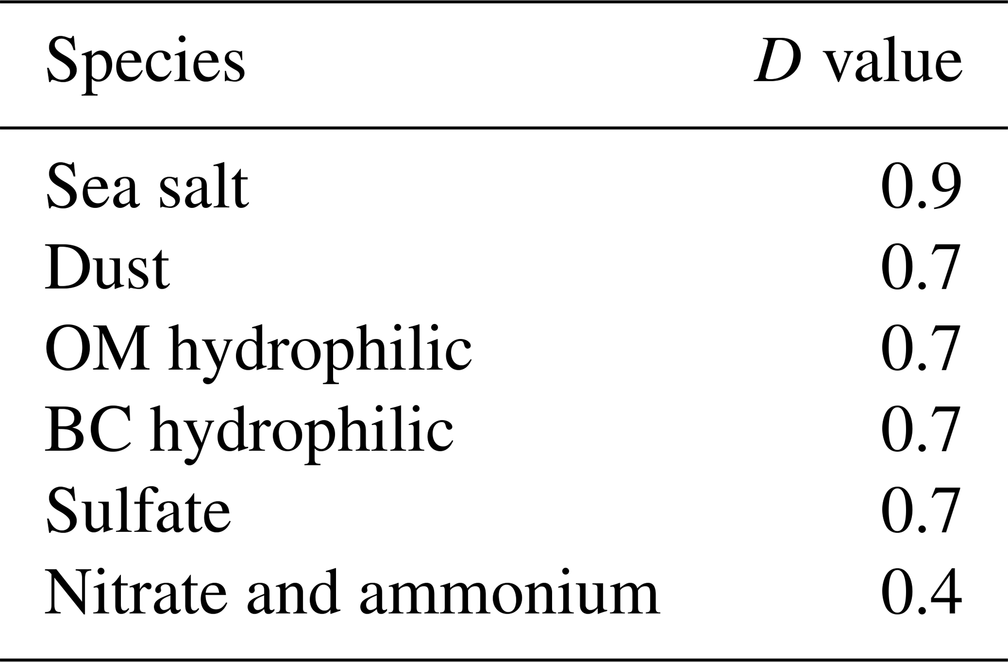
where Di is the fraction of aerosol i that is included in cloud droplets and fk is the cloud fraction at level k. The value of the parameter Di is from Reddy et al. (2005); it is indicated in Table 10. Following Giorgi and Chameides (1986), βk is the rate of conversion of cloud water to rainwater; it is computed by comparing the precipitation flux at levels k and k+1 and is written as follows:
where Pk is the sum of rain and snow precipitation fluxes at level k, qk the sum of the liquid and ice mass mixing ratio, and Δzk is the layer thickness at level k. This means that, as in M09, no distinction is made between rain and snow.
Table 10Value of the parameter D, representing the fraction of aerosol included in a cloud droplet.
5.3.2 Below-cloud wet deposition (washout)
The below-cloud scavenging rate at model k of an aerosol i is given by
where Pkl and Pki are the mean liquid and solid precipitation fluxes, respectively, ρl and ρi the water and ice density, Rl and Ri are the assumed mean radius of raindrops and snow crystals set to 1 mm, and αl and αi the efficiency with which aerosol variables are washed out by rain and snow, respectively, which account for Brownian diffusion, interception, and inertial impaction. The values used in IFS-AER for αl and αi are 0.001 and 0.01, respectively.
6.1 Optical properties
In cycle 45R1, the aerosol optical property diagnostics consist of total and fine-mode aerosol optical depth (AOD), absorption AOD (AAOD), single-scattering albedo (SSA), and the asymmetry factor, which are computed as column properties over 20 wavelengths between 340 nm and 10 µm. A lidar emulator has been implemented in IFS-AER, which also takes into account Rayleigh scattering and gaseous scattering to provide profiles of the attenuated backscattering signal from the ground or from a satellite at 355, 532, and 1064 nm. The profile of the total aerosol extinction coefficient is also output at these three wavelengths. These diagnostics use values of mass extinction, SSA, asymmetry, and the lidar ratio for each aerosol species that have been pre-computed with a standard code for Mie scattering based on Wiscombe (1980). A spherical shape is assumed for all species, with a number size distribution described by a mono-modal or bimodal log-normal function. More details on the specifics of the computation of the aerosol optical properties can be found in Bozzo et al. (2019)
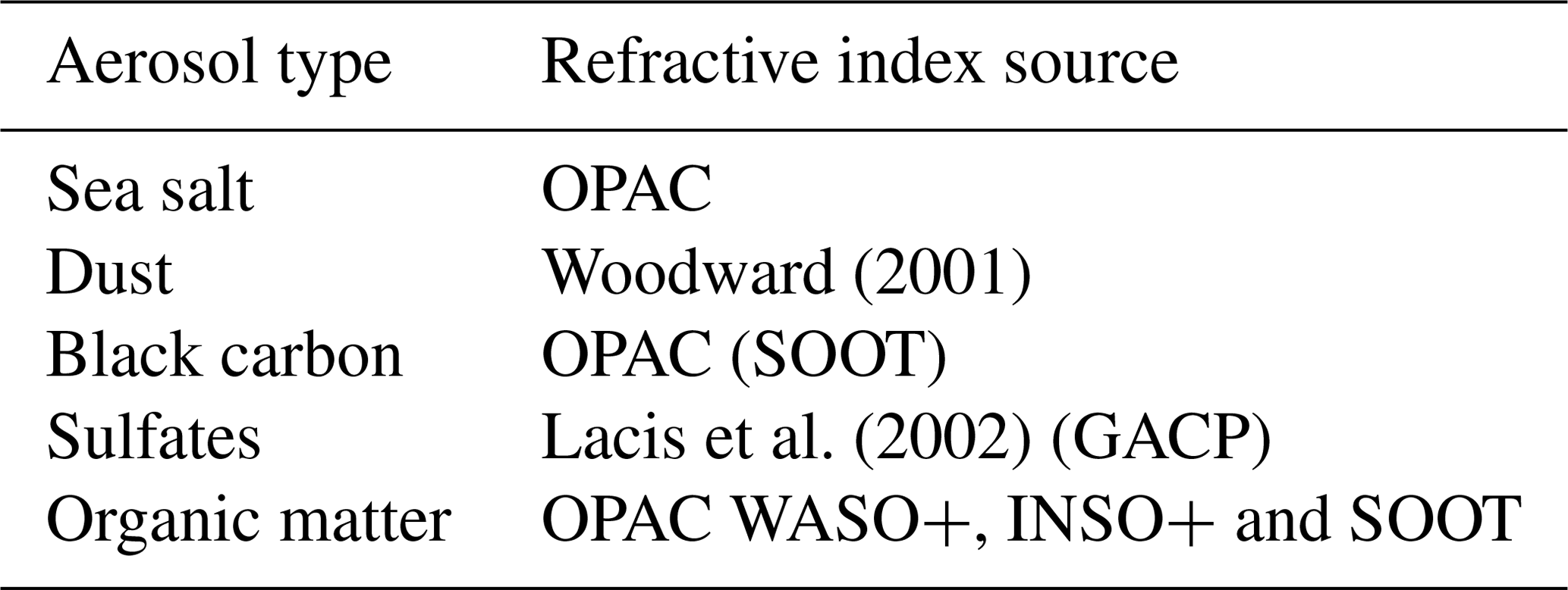
Table 11 lists the sources of the refractive indexes used in IFS-AER. For the hydrophilic types the optical properties change with the relative humidity due to the swelling of the water-soluble component in wetter environments. The growth factors applied are detailed in Table 7. A summary of the refractive index associated with each aerosol type is given in the following paragraphs.
6.1.1 Organic matter
The optical properties are based on the “continental” mixtures described in Hess et al. (1998). We use a combination of 13 % mass of insoluble soil and organic particles, 84 % water-soluble particles originated from gas-to-particle conversion containing sulfates, nitrates, and organic substances, and 3 % soot particles. The combination gives optical properties representing an average of biomass and anthropogenic organic carbon aerosols. The refractive indices and the parameters used in the particle size distribution of each component are as described in Hess et al. (1998). The hydrophobic organic matter type uses the same set of optical properties but for a fixed relative humidity of 20 %.
6.1.2 Black carbon
The refractive index used in the Mie computations is based on the OPAC SOOT model (Hess et al., 1998). At the moment the hydrophilic type of the black carbon species is not implemented and both types are treated as independent from the relative humidity. The single particle properties are integrated with a log-normal particle size distribution for sizes between 0.005 and 0.5 µm.
6.1.3 Sulfate
The refractive index is taken from the Global Aerosol Climatology Project (GACP; http://gacp.giss.nasa.gov/data_sets/, last access: 3 September 2019) and it is representative of dry ammonium sulfate.
6.1.4 Mineral dust
The large uncertainty in mineral dust composition (e.g. Colarco et al., 2014) means that it is difficult to represent the radiative properties of this species with a single refractive index fitting different parts of the world. The refractive indexes of Woodward (2001) are used, which were estimated by combining measurements from different locations and which provides the largest absorption in the visible range compared to other estimates of dust refractive indexes such as Fouquart et al. (1987) or Dubovik et al. (2002), with an imaginary refractive index at 500 nm of . The optical properties are computed individually for each of the three size intervals of the dust bins using a log-normal size distribution with limits in particle radius of 0.03, 0.55, 0.9, and 20 µm.
6.1.5 Sea salt
The refractive index for seawater is as in the OPAC database, and the optical properties are integrated across the three size ranges of the sea salt aerosol bins using bimodal log-normal distributions with limits of particle radius set at 0.03, 0.05, 5, and 20 µm as in Reddy et al. (2005).
Woodward (2001)Table 11Refractive index and parameters of the size distribution associated with each aerosol type in IFS-AER. The organic matter type is represented by a mixture of three OPAC types similar to the average continental mixture, as described in Hess et al. (1998).
6.2 PM formulae
Particulate matter smaller than 1, 2.5, and 10 µm is an important output of IFS-AER. It is computed in cycle 45R1 with the following formulae that use the mass mixing ratio from each aerosol tracer as an input, denoted for sea salt aerosol, for desert dust, [NI1,2] for nitrate, and [OM], [BC], [SU], and [AM] for organic matter, black carbon, sulfate, and ammonium, respectively.
Here, ρ is the air density. The sea salt aerosol tracers are divided by 4.3 to transform the mass mixing ratio at 80 % ambient relative humidity to the dry mass mixing ratio.
7.1 Configuration
IFS-AER was run stand-alone in cycling forecast mode, without data assimilation or coupling with the chemistry, from May 2016 to May 2018 at a resolution of TL511L60 using emissions and model options similar to the operational NRT run. Budgets are shown for June 2016 to May 2018 to allow for a month of spin-up time. The simulated AOD and PM are shown for 2017.
7.2 Budgets
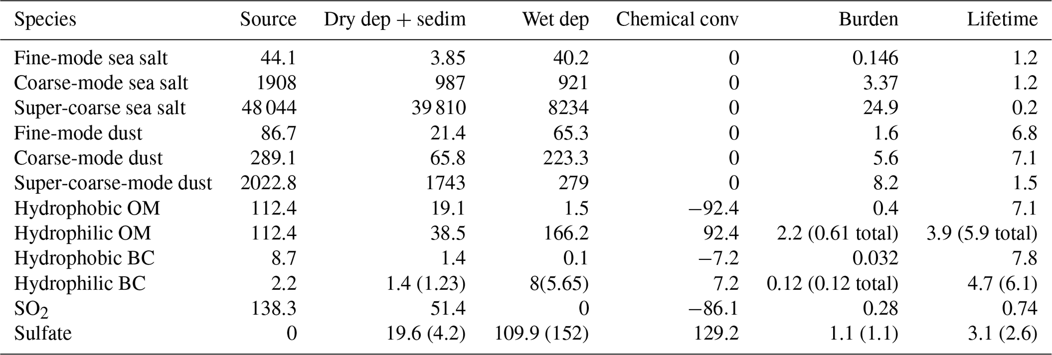
Budgets are presented in Table 12, with a comparison to values from GEOS-Chem version 9-01-03 found in Croft et al. (2014) where applicable. For both sea salt and dust, the particle size has an important impact on lifetime: the larger particles have a much shorter lifetime. Particle size also matters for the repartition of sinks between wet and dry deposition; for larger particles, dry deposition becomes preponderant. This is also because for super-coarse particles, sedimentation is also included in the dry deposition process in these tables. These numbers can be compared to the detailed budgets of GEOS-Chem presented in Croft et al. (2014). For dust, sea salt, and sulfates, the lifetime values are comparable, though slightly shorter for sulfate in GEOS-Chem with a lifetime of 2.6 d against 3.1 d in IFS-AER. For OM and BC, lifetime values are significantly shorter than in GEOS-Chem (6.1 and 5.9 d for BC and OM, respectively). The OM burden is much smaller with GEOS-Chem, which comes from the different treatment of secondary organics between the two simulations. Also, the distribution between dry and wet deposition appears to be relatively more in favour of dry deposition in IFS-AER for sulfate compared to GEOS-Chem. While the wet deposition of sulfate is lower with IFS-AER (109.9 Tg yr−1 against 152 Tg yr−1), the wet deposition of hydrophilic BC is much higher with IFS-AER at 8 Tg yr−1 against 5.65 Tg yr−1.
Table 12IFS-AER budgets for the June 2016 to May 2018 period (fluxes: Tg yr−1, burdens: Tg, lifetimes: days). Equivalents for GEOS-Chem from Croft et al. (2014) when available and comparable are indicated in parentheses.
7.3 Simulated AOD and PM
Figure 9 shows total and speciated AOD at 550 nm for 2017. The highest values are found in the dust-producing regions of North Africa, the Middle East, and the Gobi–Taklimakan, as well as in the heavily populated regions of the Indian subcontinent, eastern China, and in the most active seasonal biomass burning region in the world, which is equatorial Africa. Sea salt AOD is quite evenly spread between the mid-latitude regions where mean winds are high and the tropics where trade winds are on average less intense but with relatively more active sea salt production thanks to the dependency of sea salt production on SST. The transatlantic transport of dust produced in the western Sahara is a prominent feature, which can be compared to simulations from other models (Schepanski et al., 2009). Spatial differences in the Sahara are not very pronounced, and very active dust-producing regions such as the Bodélé depression do not appear, which could be due to a dust source function that does not discriminate enough. OM is a species that combines anthropogenic and biomass burning sources: AOD is highest over parts of China and India, mostly from secondary organics, and equatorial Africa from biomass burning. BC sources are also a combination of anthropogenic and biomass burning origin; the patterns are close to what is simulated for OM. Sulfate AOD is concentrated over heavily populated areas and a few outgassing volcanoes such as Popocatépetl in Mexico and Kilauea in Hawaii. Oceanic DMS sources bring a “background” of sulfate AOD over most oceans.
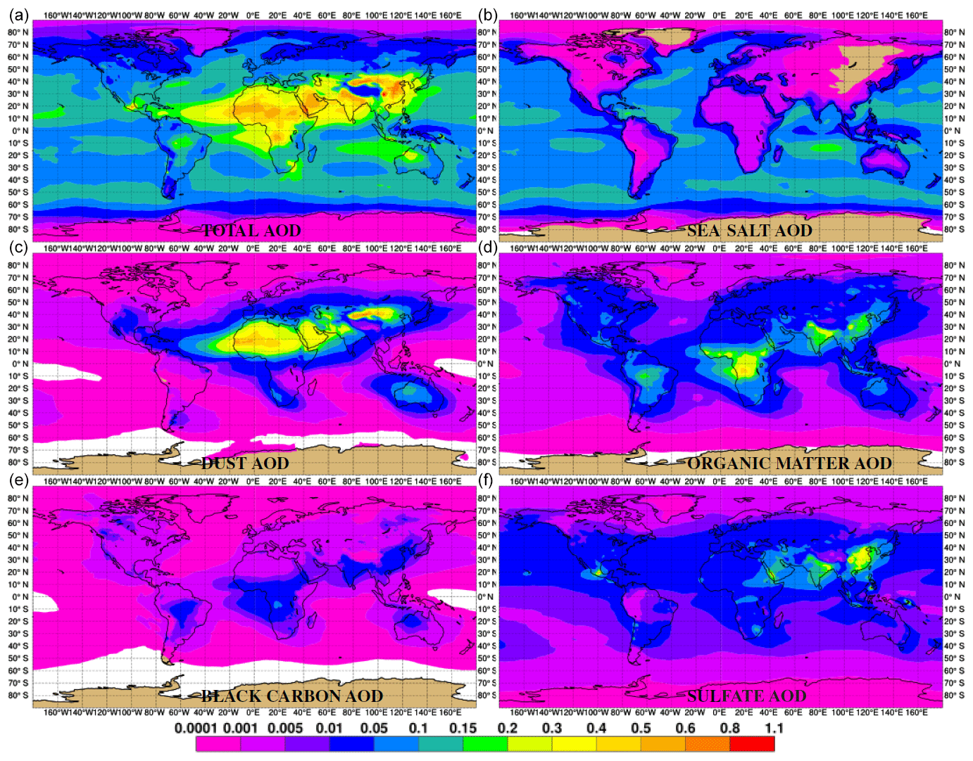
Figure 9The 2017 total (a), sea salt (b), dust (c), OM (d), BC (e), and sulfate (f) AOD at 550 nm simulated by IFS-AER cycle 45R1 in cycling forecast mode.
Figure 10 shows the global simulated PM2.5 and PM10 for 2017. Mean values over 70 to 100 µg m−3 for PM2.5 and 150 to 300 µg m−3 occur mainly over desert areas. The transatlantic transport of dust particles from the Sahara is a prominent feature, with mean PM10 values of 20–25 µg m−3 in the Caribbean islands, while in the Pacific Ocean west of Panama average PM10 values are below 10 µg m−3. Seasonal biomass burning regions such as Indonesia, Brazil, and equatorial Africa, along with a few extreme fires over eastern Siberia, the United States, and Canada, reach 70 to 100 µg m−3 for both PM2.5 and PM10; the difference between the two is negligible since OM and BC contribute their whole mass to both PM2.5 and PM10. Heavily populated areas with high pollution such as China and the Indian subcontinent also show high values, reaching average values between 40 and 70 µg m−3 for PM2.5 and up to 100–150 µg m−3 for PM10. The difference between PM2.5 and PM10 for these areas can be explained by dust sources from the Gobi and Taklimakan for China and from the Thar desert in India and Pakistan. Over most oceans and outside the influence of other species, PM2.5 and PM10 from marine aerosol reach average concentrations of 5–10 and 10–15 µg m−3, respectively. Over a large part of Europe and the United States, average values of PM2.5 and PM10 are between 5 and 15 µg m−3 and between 10 and 25 µg m−3, respectively.
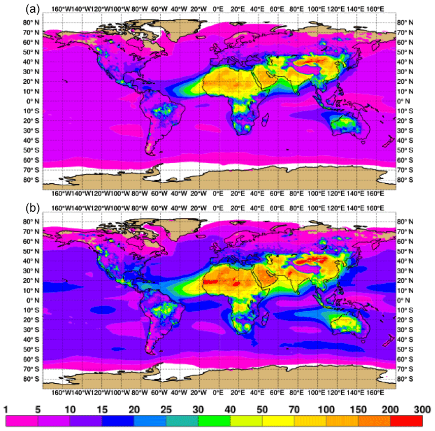
Figure 10Global 2017 near-surface PM2.5 (a) and PM10 (b) (µg m−3) simulated by IFS-AER cycle 45R1 in cycling forecast mode.
In this section, a short evaluation of the simulated AOD against observations from the Aerosol Robotic Network (AERONET; Holben et al., 1998) is shown, as well as of PM2.5 and PM10 against observations from the AirNow and AirBase networks in the United States and Europe, respectively. The simulations evaluated here consist of 24 h cycling forecasts with meteorological initial conditions provided by an analysis and aerosol and chemical initial conditions provided by the previous forecast. No aerosol data assimilation was used in the simulations that have been evaluated in this section. An evaluation of such a simulation with cycle 45R1 using the same configuration and resolution (TL511L60) as the operational forecasts is presented first. A comparison of the skill scores between stand-alone and coupled IFS-CB05 simulations with cycle 45R1 is then made. Finally, the skill scores of simulations with cycles 40R2 and 45R1 are compared with simulations using similar resolution (TL159L60) and emissions. Cycle 40R2 was chosen because it was used in the CAMS interim ReAnalysis and because the changes between cycle 32R2, described in Morcrette et al. (2009), and cycle 40R2 are limited as far as aerosols are concerned. Because of upgrades in the ECMWF high-performance computing facility, it is no longer possible to run simulations of the original cycle 32R2. This is not intended as a full evaluation, which would require a much more thorough validation of the output of IFS-AER, but rather to show that the model performs relatively well for the headline CAMS products.
8.1 Summary
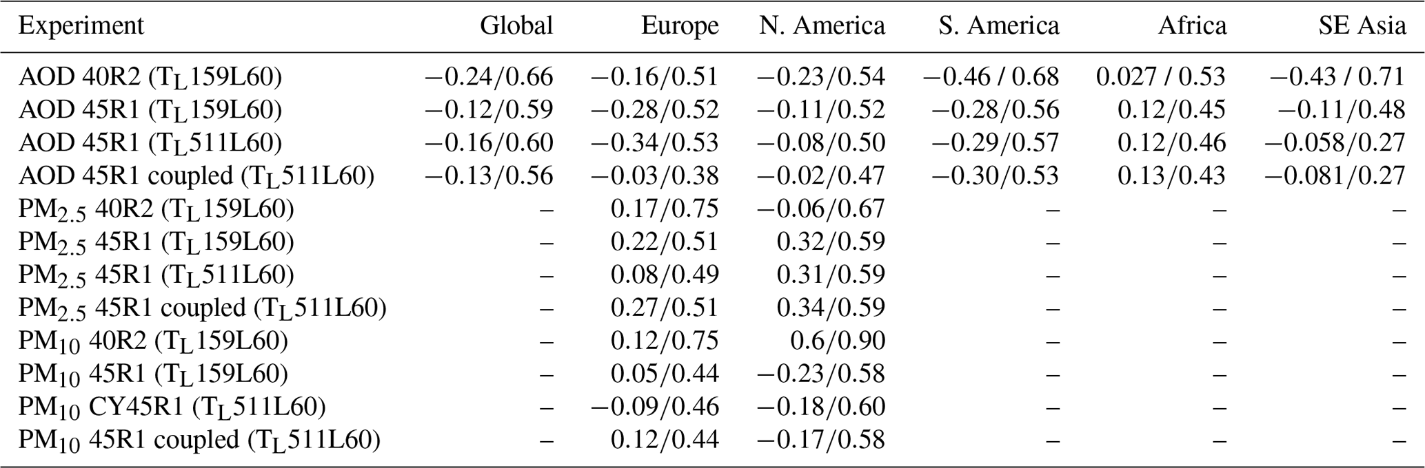
Table 13 shows a summary of global and regional skill scores for AOD at 500 nm and PM for a year of simulation for the four experiments described above. The modified normalized mean bias (MNMB) and fractional gross error (FGE) are shown so that the skill of the model in simulating relatively low AOD values is not overlooked. MNMB varies by −2, and B and is defined by the following equation for a population of N forecasts fi and observations oi:
FGE varies between 0 (best) and 2 (worst) and is defined as
For all regions and for AOD at 500 nm, PM2.5, and PM10, the FGE is improved by cycle 45R1 compared to 40R2 at a similar resolution, sometimes by a large margin: global FGE on AOD at 500 nm is decreased by more than 10 %. The only exception is over Europe where the mean FGE for AOD is nearly similar between the two cycles. Bias, as measured by MNMB, is improved nearly everywhere except over Europe and Africa for AOD and North America for PM2.5. Interestingly, the 45R1 simulation using the operational resolution of TL511L60 shows an improved MNMB for AOD and more markedly for PM2.5 compared to the 45R1 simulation at TL159L60. The simulation with cycle 45R1 coupled with IFS-CB05 shows a small improvement compared to stand-alone CY45R1 at a global scale. However, regional AOD scores are notably improved with the coupled simulation, especially over Europe, where FGE is reduced from 0.53 to 0.38 and where the negative bias is nearly eliminated.
Table 13Average over 1 May 2016 to 1 May 2017 of the modified normalized mean bias (MNMB) ∕ fractional gross error (FGE) of daily AOD at 500 nm and PM from the experiments described in this section. AOD observations are from AERONET level 2; European PM observations are from 65 PM2.5 and 138 PM10 background rural AirBase stations; North American PM observations are from 1006 PM2.5 stations and 336 PM10 stations.
8.2 Evaluation against AERONET
Figures 11 gives an indication of how the model compared to AERONET observations for daily AOD forecasts, globally and over Europe, in its stand-alone and coupled to the chemistry (including nitrates) configurations. When coupled to the chemistry, sulfate oxidation rates are provided by IFS-CB05 and are generally lower than the rates computed by the simple scheme of IFS-AER. The lower sulfate burden and surface concentrations are compensated for by contributions from nitrate and ammonium. The global MNMB is generally negative but slightly less so for the coupled version, with values usually between −0.1 and −0.2. Over Europe, MNMB with the stand-alone cycle 45R1 is more negative, from −0.2 to −0.6; the improvement is significant with the coupled configuration, with MNMB only slightly negative in general. Global FGE is between 0.5 and 0.7 generally but slightly less with the coupled configuration. European FGE is much improved by the coupled configuration, decreasing from 0.5–0.7 on average to 0.3–0.5.
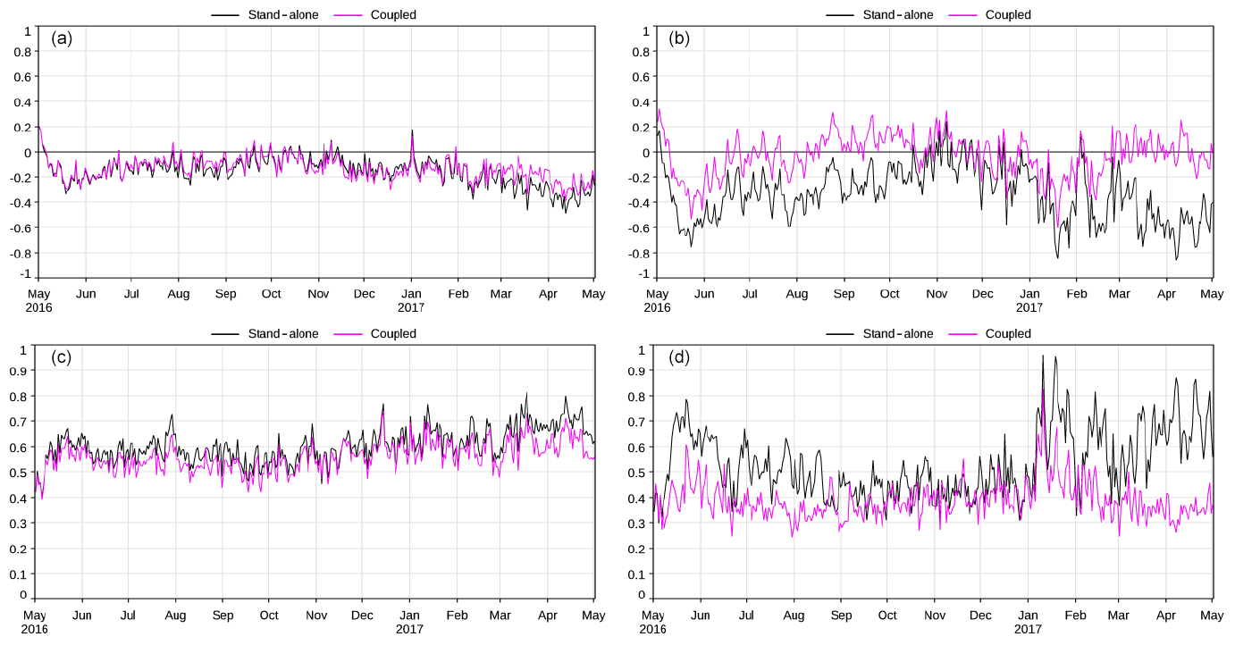
Figure 11Global (a, c) and European (b, d) modified normalized mean bias (MNMB; a, b) and fractional gross error (FGE; c, d) of daily AOD at 500 nm simulated by stand-alone (black) and coupled (violet) IFS-AER cycle 45R1 against observations from AERONET.
8.3 Evaluation against PM observations
In this section, simulations of near-surface PM2.5 and PM10 are evaluated against observations from two regional networks: the AirNow network, which gathers observations mostly over the United States and Canada, and AirBase, the European Air Quality Database operated by the European Environment Agency (EEA), which gathers observations over Europe. As metadata were not available for AirNow observations, data from all sites (1036 for PM2.5 and 354 for PM10 in 2017) are used, which means that urban, suburban, and rural stations are included in the scores. Similarly, the observations may not be representative of background pollution or closer to traffic sources. For the AirBase observations, for which site information was available, the chosen focus was on scores vs. background rural stations (62 stations in all). Because of the relatively coarse horizontal resolution of the simulation (about 40 km), urban areas cannot be realistically represented and this will lead to a low bias compared to observations, caused not from issues in the model or in emissions but mostly from resolution. Figures 12 and 13 show the result of the evaluation against the AirNow and the AirBase observations, respectively, for the stand-alone and the coupled configurations.
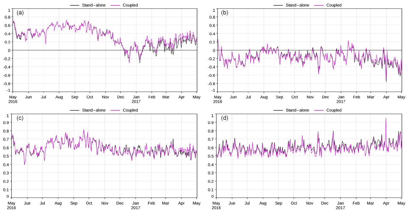
Figure 12MNMB (a, b) and FGE (c, d) of daily near-surface PM2.5 (a, c) and PM10 (b, d) (µg m−3) simulated by stand-alone (black) and coupled (violet) cycle 45R1 against North American observations from the AirNow network.
Observed PM2.5 at all AirNow stations shows higher values during the summer months, reaching 30 µg m−3 in early September. These high values ware generally caused by fire events. IFS-AER generally overestimates PM2.5 significantly, with MNMB between 0.2 and 0.6 except during the winter of 2016–2017. This overestimation is mainly caused by SOA emissions at the surface, which contribute to a large fraction of PM2.5, and to the fact that emissions from biomass burning are released at the surface, which can increase PM2.5 forecasts to very high values during fire events. The FGE against PM2.5 observations over North America stands at 0.5–0.7, with relatively little variation. Simulated PM10 is generally biased low in contrast to PM2.5, and the FGE is also slightly higher , with values of 0.5–0.8. Both MNMB and FGE are relatively similar for the stand-alone and coupled configurations.
Compared to AirBase observations (Fig. 13), PM2.5 and PM10 show a negative MNMB during most of January and February 2017 at −0.4 to −0.8 for the stand-alone configuration. For the rest of the year, MNMB is positive for PM2.5 but with values hovering around 0.2 for stand-alone and 0.4 when running coupled with the chemistry. The MNMB of PM10 simulated with the stand-alone configuration is slightly negative from May to September 2016, with values between 0 and −0.2, positive during autumn, and very negative during January–February 2017, possibly caused by the underestimation of the surface concentration of anthropogenic aerosols during the mostly anticyclonic conditions of this period. The MNMB of PM10 is lifted upwards by ∼0.25 on average and becomes generally positive when running coupled with the chemistry. The FGEs of simulated PM2.5 and PM10 are quite close and are generally between 0.4 and 0.7, with higher values during parts of January and February 2017 probably associated with pollution events. Interestingly, the FGE is generally higher when coupled with the chemistry but lower during the January–February 2017 spikes, showing that these pollution events are better simulated when the coupling with the chemistry is used.
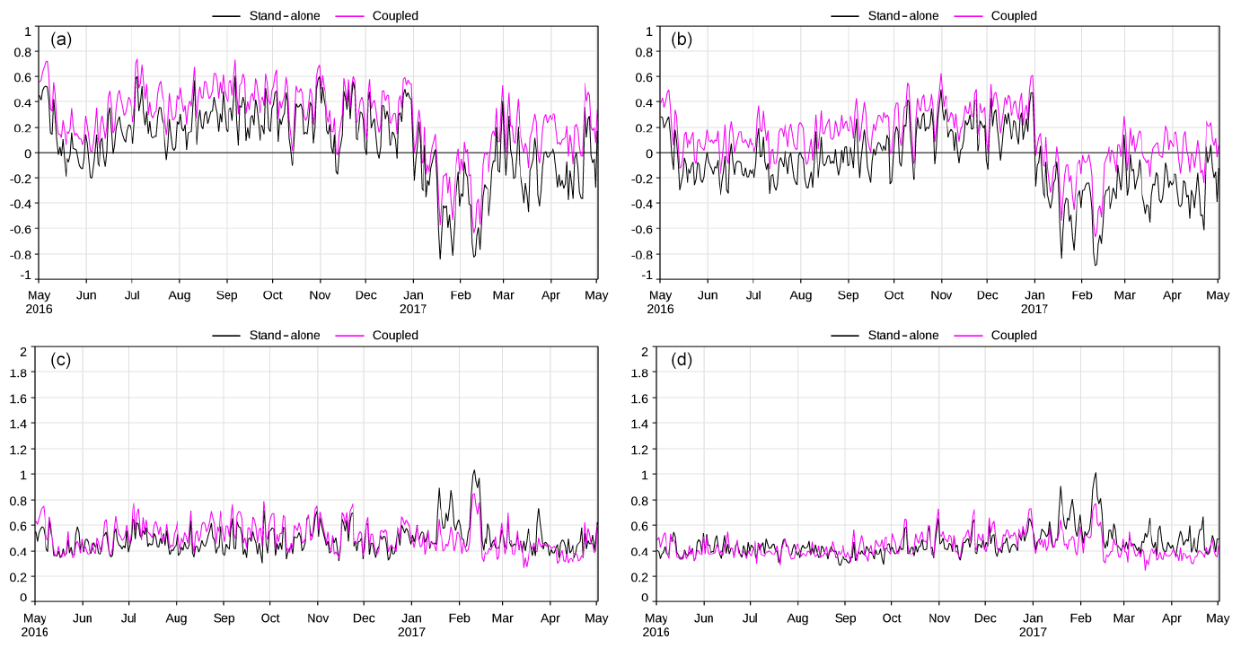
Figure 13MNMB (a, b) and FGE (c, d) of daily near-surface PM2.5 (a, c) and PM10 (b, d) (µg m−3) simulated by stand-alone (black) and coupled (violet) cycle 45R1 against European observations from the AirBase network.
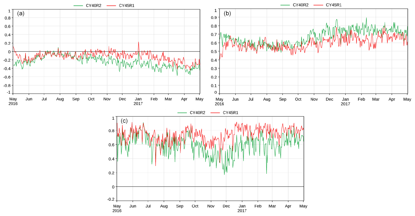
Figure 14MNMB (a), FGE (b), and spatial correlation (c) of daily AOD at 500–550 nm simulated by cycles 40R2 (green) and 45R1 (red) against global observations from AERONET.
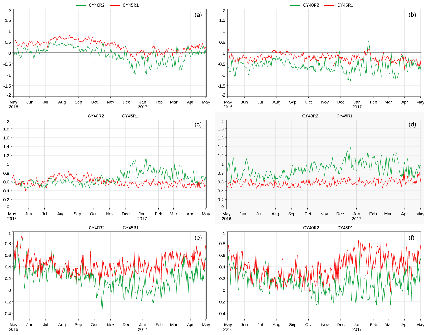
Figure 15MNMB (a, b), FGE (c, d), and spatial correlation (e, f) of daily near-surface PM2.5 (a, c, e) and PM10 (b, d, f) (µg m−3) simulated by cycles 40R2 (green) and 45R1 (red) against observations in the United States from the AirNow network.
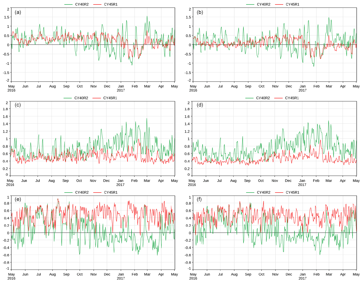
Figure 16MNMB (a, b), FGE (c, d), and spatial correlation (e, f) of daily near-surface PM2.5 (a, c, e) and PM10 (b, d, f) (µg m−3) simulated by cycles 40R2 (green) and 45R1 (red) against observations of background rural stations in Europe from the AirBase network.
8.4 Comparison with IFS-AER cycle 40R2
This section aims to give an initial evaluation of the impact of the model upgrades between cycles 40R2 and 45R1. To achieve this, the control run (i.e. without data assimilation) of the CAMS interim ReAnalysis following Flemming et al. (2017) is used, and a simulation with cycle 45R1 in stand-alone mode using the same fixed emissions (except for the new SOA emissions) and the same horizontal resolution (TL159) was carried out. The latter simulation covers the May–December 2016 period. Skill scores of daily AOD vs. AERONET observations and of daily near-surface PM2.5 and PM10 vs. observations from the AirBase and AirNow networks were then computed and are shown in Figs. 14, 15, and 16. Compared to cycle 40R2, 45R1 brings an important improvement in the skill of AOD forecasts, as measured by MNMB, FGE, and correlation. MNMB is generally above −0.1 for 45R1. The global FGE is significantly reduced and RMSE (not shown) is at times more than halved by 45R1 compared to 40R2. The spatial correlation is also generally higher with cycle 45R1 compared to 40R2. The development that had the most impact on skill scores against AERONET is the implementation of a new SOA source in cycle 43R1, which led to a significant improvement of both bias and RMSE. Using the ZH01 dry deposition scheme also improved scores. The new G14 sea salt aerosol scheme had little impact on AOD scores against AERONET or on PM skill scores, but it notably improved the bias and RMSE versus MODIS AOD. Skill scores of the global PM simulations are also generally improved, except for PM2.5 over North America, for which the MNMB and the FGE during summer are degraded by cycle 45R1 compared to 40R2. The correlation is nonetheless improved. This degradation is caused by the new source of SOA, which is associated with high PM values over North America and an unrealistic diurnal cycle. PM10 is generally underestimated over North America but less so with 45R1. This is associated with a lower error and a much higher correlation of simulations with observations. PM forecasts over Europe are significantly improved by cycle 45R1 compared to 40R2. The improvement is especially marked for PM10, for which the RMSE (not shown) is reduced by more than a factor of 3.
IFS-AER is a simple and low-cost scheme that aims to represent the major atmospheric aerosol species. Because of this simplicity, many processes such as internal mixing, coagulation, and nucleation are not explicitly represented. Despite this, IFS-AER achieves reasonable skill in forecasting AOD and PM. The skill for the headline products of the operational CAMS system, AOD and PM, was improved considerably (except for PM2.5 over North America) from cycle 40R2 to 45R1. The tendency has been towards a system that is more integrated with the other components of the IFS, particularly atmospheric chemistry, with the possibility to run with integrated sulfur and ammonia cycles. The coupling with IFS-CB05 generally improves the error of the forecasts of IFS-AER, except for European PM simulations. This also makes the skill of IFS-AER more dependent on the evolution of IFS-CB05.
Compared to the original implementation as described in Morcrette et al. (2009), many components of IFS-AER have been reviewed, and two new species (nitrate and ammonium) were added. Some parameterizations, on the other hand, such as dust production and wet scavenging are essentially similar in cycle 45R1 as in M09. Future upgrades will aim to address some of the shortcomings noted in the model evaluation. The currently operational cycle 46R1, for which a description of the changes can be found at https://atmosphere.copernicus.eu/node/472 (last access: 4 September 2019), includes an upgrade of the dust emission and scavenging schemes as well as the use of biomass burning injection heights for aerosols and trace gas fire emissions. IFS-AER is running in cycle 46R1 coupled with the chemistry, with the new nitrate and ammonium species. The treatment of secondary organics is also very simplistic and leads to an unrealistic diurnal cycle in PM simulations regionally. In the longer term, the possibility to use SOA production rates provided by the chemistry scheme will be given.
Model codes developed at the ECMWF are the intellectual property of the ECMWF and its member states, and therefore the IFS code is not publicly available. ECMWF member-state weather services and their approved partners will get access granted. Access to a reduced version of the IFS code, not including the aerosol component, may be obtained from the ECMWF under an OpenIFS licence.
SR drafted the paper; SR, ZK, and JF maintained and carried out developments on IFS-AER; OB developed the LMD-LOA model from which IFS-AER was adapted; JJM carried out developments on IFS-AER up to cycle 38R2; PN and MM contributed to the desert dust and sea salt parameterizations, ABo to the optical properties part, and VH to the coupling to IFS-CB05. MA, ABe, RE, and VHP contributed to drafting and revising this article.
The authors declare that they have no conflict of interest.
This work is supported by the Copernicus Atmospheric Monitoring Services (CAMS) programme managed by the ECMWF on behalf of the European Commission. The authors would also like to thank NASA, the European Environment Agency, the AirNow network, and the United States Environmental Protection Agency (EPA) for making the MODIS, AirBase, AirNow, and CASTNET data publicly available.
This paper was edited by Slimane Bekki and reviewed by three anonymous referees.
Agustí-Panareda, A., Massart, S., Chevallier, F., Boussetta, S., Balsamo, G., Beljaars, A., Ciais, P., Deutscher, N. M., Engelen, R., Jones, L., Kivi, R., Paris, J.-D., Peuch, V.-H., Sherlock, V., Vermeulen, A. T., Wennberg, P. O., and Wunch, D.: Forecasting global atmospheric CO2, Atmos. Chem. Phys., 14, 11959–11983, https://doi.org/10.5194/acp-14-11959-2014, 2014. a
Agusti-Panareda, A., Diamantakis, M., Bayona, V., Klappenbach, F., and Butz, A.: Improving the inter-hemispheric gradient of total column atmospheric CO2 and CH4 in simulations with the ECMWF semi-Lagrangian atmospheric global model, Geosci. Model Dev., 10, 1–18, https://doi.org/10.5194/gmd-10-1-2017, 2017. a
Baklanov, A., Schlünzen, K., Suppan, P., Baldasano, J., Brunner, D., Aksoyoglu, S., Carmichael, G., Douros, J., Flemming, J., Forkel, R., Galmarini, S., Gauss, M., Grell, G., Hirtl, M., Joffre, S., Jorba, O., Kaas, E., Kaasik, M., Kallos, G., Kong, X., Korsholm, U., Kurganskiy, A., Kushta, J., Lohmann, U., Mahura, A., Manders-Groot, A., Maurizi, A., Moussiopoulos, N., Rao, S. T., Savage, N., Seigneur, C., Sokhi, R. S., Solazzo, E., Solomos, S., Sørensen, B., Tsegas, G., Vignati, E., Vogel, B., and Zhang, Y.: Online coupled regional meteorology chemistry models in Europe: current status and prospects, Atmos. Chem. Phys., 14, 317–398, https://doi.org/10.5194/acp-14-317-2014, 2014. a
Bechtold, P. and Bidlot, J.-R.: Parametrization of convective gusts, ECMWF newsletter, 119, 15–18, 2009. a
Bechtold, P., Semane, N., Lopez, P., Chaboureau, J.-P., Beljaars, A., and Bormann, N.: Representing Equilibrium and nonequilibrium convection in large-scale models, J. Atmos. Sci., 71, 734–753, 2014. a
Beljaars, A. and Viterbo, P.: The role of the boundary layer in a numerical weather prediction model, in: Clear and cloudy boundary layers, edited by: Holtslag, A. A. M. and Duynkerke, P., North Holland Publishers, 287–304, 1998. a, b, c
Bellouin, N., Boucher, O., Haywood, J., and Shekar Reddy, M.: Global estimate of aerosol direct radiative forcing from satellite measurements, Nature, 438, 1138–1141, 2005. a
Bellouin, N., Rae, J., Jones, A., Johnson, C., Haywood, J., and Boucher, O.: Aerosol forcing in the Climate Model Intercomparison Project (CMIP5) simulations by HadGEM2-ES and the role of ammonium nitrate, J. Geophys. Res.-Atmos., 116, D20206, https://doi.org/10.1029/2011JD016074, 2011b. a, b
Benedetti, A. and Vitart, F.: Can the Direct Effect of Aerosols Improve Subseasonal Predictability?, Mon. Weather Rev., 146, 3481–3498, 2018. a
Benedetti, A., Morcrette, J.-J., Boucher, O., Dethof, A., Engelen, R., Fisher, M., Flentje, H., Huneeus, N., Jones, L., Kaiser, J., Kinne, S., Mangold, A., Razinger, M., Simmons, A. J., and Suttie, M.: Aerosol analysis and forecast in the European centre for medium-range weather forecasts integrated forecast system: 2. Data assimilation, J. Geophys. Res.-Atmos., 114, D13205, https://doi.org/10.1029/2008JD011235, 2009. a, b, c
Bian, H., Chin, M., Hauglustaine, D. A., Schulz, M., Myhre, G., Bauer, S. E., Lund, M. T., Karydis, V. A., Kucsera, T. L., Pan, X., Pozzer, A., Skeie, R. B., Steenrod, S. D., Sudo, K., Tsigaridis, K., Tsimpidi, A. P., and Tsyro, S. G.: Investigation of global particulate nitrate from the AeroCom phase III experiment, Atmos. Chem. Phys., 17, 12911–12940, https://doi.org/10.5194/acp-17-12911-2017, 2017. a
Boucher, O., Pham, M., and Venkataraman, C.: Simulation of the atmospheric sulfur cycle in the Laboratoire de Meteorologie Dynamique general circulation model: Model description, model evaluation, and global and European budgets, Note Scientifique de l'IPSL, 23, 27 pp., 2002. a
Bozzo, A., Benedetti, A., Flemming, J., Kipling, Z., and Rémy, S.: An aerosol climatology for global models based on the tropospheric aerosol scheme in the Integrated Forecasting System of ECMWF, Geosci. Model Dev. Discuss., https://doi.org/10.5194/gmd-2019-149, in review, 2019. a, b, c, d
Brasseur, G. P., Xie, Y., Petersen, A. K., Bouarar, I., Flemming, J., Gauss, M., Jiang, F., Kouznetsov, R., Kranenburg, R., Mijling, B., Peuch, V.-H., Pommier, M., Segers, A., Sofiev, M., Timmermans, R., van der A, R., Walters, S., Xu, J., and Zhou, G.: Ensemble forecasts of air quality in eastern China – Part 1: Model description and implementation of the MarcoPolo–Panda prediction system, version 1, Geoscientific Model Development, 12, 33–67, 2019. a, b
Canagaratna, M. R., Jimenez, J. L., Kroll, J. H., Chen, Q., Kessler, S. H., Massoli, P., Hildebrandt Ruiz, L., Fortner, E., Williams, L. R., Wilson, K. R., Surratt, J. D., Donahue, N. M., Jayne, J. T., and Worsnop, D. R.: Elemental ratio measurements of organic compounds using aerosol mass spectrometry: characterization, improved calibration, and implications, Atmos. Chem. Phys., 15, 253–272, https://doi.org/10.5194/acp-15-253-2015, 2015. a
Chin, M., Ginoux, P., Kinne, S., Torres, O., Holben, B., Duncan, B., and Martin, R.: Tropospheric aerosol optical thickness from the GOCART model and comparisons with satellite and Sun photometer measurements, J. Atmos. Sci., 59, 461–483, 2002. a
Colarco, P.: The NASA GEOS-5 Aerosol Forecasting System, MACC Conference, Driebergen, the Netherlands, 2011. a
Colarco, P. R., Nowottnick, E., Randles, C. A., Yi, B., Yang, P., Kim, K.-M., Smith, J. A., and Bardeen, C. G.: Impact of radiatively interactive dust aerosols in the NASA GEOS-5 climate model: Sensitivity to dust particle shape and refractive index, J. Geophys. Res.-Atmos., 119, 753–786, 2014. a
Croft, B., Pierce, J. R., and Martin, R. V.: Interpreting aerosol lifetimes using the GEOS-Chem model and constraints from radionuclide measurements, Atmos. Chem. Phys., 14, 4313–4325, https://doi.org/10.5194/acp-14-4313-2014, 2014. a, b, c
Curran, M. A. J. and Jones, G. B.: Dimethyl sulfide in the Southern Ocean: Seasonality and flux, J. Geophys. Res.-Atmos., 105, 20451–20459, https://doi.org/10.1029/2000JD900176, 2000. a
Dentener, F., Kinne, S., Bond, T., Boucher, O., Cofala, J., Generoso, S., Ginoux, P., Gong, S., Hoelzemann, J. J., Ito, A., Marelli, L., Penner, J. E., Putaud, J.-P., Textor, C., Schulz, M., van der Werf, G. R., and Wilson, J.: Emissions of primary aerosol and precursor gases in the years 2000 and 1750 prescribed data-sets for AeroCom, Atmos. Chem. Phys., 6, 4321–4344, https://doi.org/10.5194/acp-6-4321-2006, 2006. a
Diamantakis, M. and Flemming, J.: Global mass fixer algorithms for conservative tracer transport in the ECMWF model, Geosci. Model Dev., 7, 965–979, https://doi.org/10.5194/gmd-7-965-2014, 2014. a
Dubovik, O., Holben, B., Eck, T., Smirnov, A., Kaufman, Y., King, M., Tanre, D., and Slutsker, I.: Variability of absorption and optical properties of key aerosol types observed in worldwide locations, J. Atmos. Sci., 59, 590–608, 2002. a
Eatough, D., Caka, F., and Farber, R.: The Conversion of SO2 to Sulfate in the Atmosphere, Isr. J. Chem., 34, 301–314, https://doi.org/10.1002/ijch.199400034, 1994. a
Engelen, R. J., Serrar, S., and Chevallier, F.: Four-dimensional data assimilation of atmospheric CO2 using AIRS observations, J. Geophys. Res.-Atmos., 114, D03303, https://doi.org/10.1029/2008JD010739, 2009. a
Errera, Q., Daerden, F., Chabrillat, S., Lambert, J. C., Lahoz, W. A., Viscardy, S., Bonjean, S., and Fonteyn, D.: 4D-Var assimilation of MIPAS chemical observations: ozone and nitrogen dioxide analyses, Atmos. Chem. Phys., 8, 6169–6187, https://doi.org/10.5194/acp-8-6169-2008, 2008. a
Fairlie, T. D., Jacob, D. J., Dibb, J. E., Alexander, B., Avery, M. A., van Donkelaar, A., and Zhang, L.: Impact of mineral dust on nitrate, sulfate, and ozone in transpacific Asian pollution plumes, Atmos. Chem. Phys., 10, 3999–4012, https://doi.org/10.5194/acp-10-3999-2010, 2010. a, b
Fan, J., Y. W., Rosenfeld, D., and Liu, X.: Review of aerosol–cloud interactions: Mechanisms, significance, and challenges, J. Atmos. Sci., 73, 4221–4252, 2016. a
Flemming, J., Inness, A., Flentje, H., Huijnen, V., Moinat, P., Schultz, M. G., and Stein, O.: Coupling global chemistry transport models to ECMWF's integrated forecast system, Geosci. Model Dev., 2, 253–265, https://doi.org/10.5194/gmd-2-253-2009, 2009. a
Flemming, J., Huijnen, V., Arteta, J., Bechtold, P., Beljaars, A., Blechschmidt, A.-M., Diamantakis, M., Engelen, R. J., Gaudel, A., Inness, A., Jones, L., Josse, B., Katragkou, E., Marecal, V., Peuch, V.-H., Richter, A., Schultz, M. G., Stein, O., and Tsikerdekis, A.: Tropospheric chemistry in the Integrated Forecasting System of ECMWF, Geosci. Model Dev., 8, 975–1003, https://doi.org/10.5194/gmd-8-975-2015, 2015. a, b, c, d, e, f, g
Flemming, J., Benedetti, A., Inness, A., Engelen, R. J., Jones, L., Huijnen, V., Remy, S., Parrington, M., Suttie, M., Bozzo, A., Peuch, V.-H., Akritidis, D., and Katragkou, E.: The CAMS interim Reanalysis of Carbon Monoxide, Ozone and Aerosol for 2003–2015, Atmos. Chem. Phys., 17, 1945–1983, https://doi.org/10.5194/acp-17-1945-2017, 2017. a, b, c, d
Fouquart, Y., Bonnel, B., Brogniez, G., Buriez, J., Smith, L., Morcrette, J., and Cerf, A.: Observations of Saharan aerosols: Results of ECLATS field experiment. Part II: Broadband radiative characteristics of the aerosols and vertical radiative flux divergence, J. Clim. Appl. Meteorol., 26, 38–52, 1987. a
Freitas, S. R., Longo, K. M., Trentmann, J., and Latham, D.: Technical Note: Sensitivity of 1-D smoke plume rise models to the inclusion of environmental wind drag, Atmos. Chem. Phys., 10, 585–594, https://doi.org/10.5194/acp-10-585-2010, 2010. a
Fromm, M., Bevilacqua, R., Servranckx, R., Rosen, J., Thayer, J. P., Herman, J., and Larko, D.: Pyro-cumulonimbus injection of smoke to the stratosphere: observations and impact of a super blowup in northwestern Canada on 3–4 August 1998, J. Geophys. Res.-Atmos., 110, D08205, https://doi.org/10.1029/2004JD005350, 2005. a
Gidden, M. J., Riahi, K., Smith, S. J., Fujimori, S., Luderer, G., Kriegler, E., van Vuuren, D. P., van den Berg, M., Feng, L., Klein, D., Calvin, K., Doelman, J. C., Frank, S., Fricko, O., Harmsen, M., Hasegawa, T., Havlik, P., Hilaire, J., Hoesly, R., Horing, J., Popp, A., Stehfest, E., and Takahashi, K.: Global emissions pathways under different socioeconomic scenarios for use in CMIP6: a dataset of harmonized emissions trajectories through the end of the century, Geosci. Model Dev., 12, 1443–1475, https://doi.org/10.5194/gmd-12-1443-2019, 2019. a, b
Ginoux, P., Chin, M., Tegen, I., Prospero, J. M., Holben, B., Dubovik, O., and Lin, S.-J.: Sources and distributions of dust aerosols simulated with the GOCART model, J. Geophys. Res.-Atmos., 106, 20255–20273, 2001. a, b
Ginoux, P., Prospero, J. M., Gill, T. E., Hsu, N. C., and Zhao, M.: Global-scale attribution of anthropogenic and natural dust sources and their emission rates based on MODIS Deep Blue aerosol products, Rev. Geophys., 50, RG3005, https://doi.org/10.1029/2012RG000388, 2012. a
Giorgi, F. and Chameides, W. L.: Rainout lifetimes of highly soluble aerosols and gases as inferred from simulations with a general circulation model, J. Geophys. Res., 91, 367–376, 1986. a
Granier, C., Bessagnet, B., Bond, T., D'Angiola, A., van der Gon, H. D., Frost, G. J., Heil, A., Kaiser, J. W., Kinne, S., Klimont, Z., Kloster, S., Lamarque, J.-F., Liousse, C., Masui, T., Meleux, F., Mieville, A., Ohara, T., Raut, J.-C., Riahi, K., Schultz, M. G., Smith, S. J., Thomson, A., van Aardenne, J., van der Werf, G. R., and van Vuuren, D. P.: Evolution of anthropogenic and biomass burning emissions of air pollutants at global and regional scales during the 1980–2010 period, Climate Change, 109, 163–190, 2011. a, b
Grythe, H., Ström, J., Krejci, R., Quinn, P., and Stohl, A.: A review of sea-spray aerosol source functions using a large global set of sea salt aerosol concentration measurements, Atmos. Chem. Phys., 14, 1277–1297, https://doi.org/10.5194/acp-14-1277-2014, 2014. a, b, c
Hallquist, M., Wenger, J. C., Baltensperger, U., Rudich, Y., Simpson, D., Claeys, M., Dommen, J., Donahue, N. M., George, C., Goldstein, A. H., Hamilton, J. F., Herrmann, H., Hoffmann, T., Iinuma, Y., Jang, M., Jenkin, M. E., Jimenez, J. L., Kiendler-Scharr, A., Maenhaut, W., McFiggans, G., Mentel, Th. F., Monod, A., Prévôt, A. S. H., Seinfeld, J. H., Surratt, J. D., Szmigielski, R., and Wildt, J.: The formation, properties and impact of secondary organic aerosol: current and emerging issues, Atmos. Chem. Phys., 9, 5155–5236, https://doi.org/10.5194/acp-9-5155-2009, 2009. a
Hauglustaine, D. A., Balkanski, Y., and Schulz, M.: A global model simulation of present and future nitrate aerosols and their direct radiative forcing of climate, Atmos. Chem. Phys., 14, 11031–11063, https://doi.org/10.5194/acp-14-11031-2014, 2014. a, b, c, d, e, f
Hess, M., Koepke, P., and Schult, I.: Optical Properties of Aerosols and Clouds: The Software Package OPAC., B. Am. Meteorol. Soc., 79, 831–844, 1998. a, b, c, d, e
Hodzic, A., Kasibhatla, P. S., Jo, D. S., Cappa, C. D., Jimenez, J. L., Madronich, S., and Park, R. J.: Rethinking the global secondary organic aerosol (SOA) budget: stronger production, faster removal, shorter lifetime, Atmos. Chem. Phys., 16, 7917–7941, https://doi.org/10.5194/acp-16-7917-2016, 2016. a, b
Hogan, R. J. and Bozzo, A.: A Flexible and Efficient Radiation Scheme for the ECMWF Model, J. Adv. Model. Earth Sy., 10, 1990–2008, https://doi.org/10.1029/2018MS001364, 2018. a
Holben, B. N., Eck, T., Slutsker, I., Tanre, D., Buis, J., Setzer, A., Vermote, E., Reagan, J., Kaufman, Y., Nakajima, T., Lavenu, F., Jankowiak, I., and Smirnov, A.: AERONET-A federated instrument network and data archive for aerosol characterization, Remote Sens. Environ., 66, 1–16, 1998. a, b
Hollingsworth, A., Engelen, R. J., T. C., Benedetti, A., Boucher, O., Chevallier, F., Dethof, A., Elbern, H., Eskes, H., Flemming, J., Granier, C., Kaiser, J. W., Morcrette, J.-J., Rayner, P., Peuch, V. H., Rouil, L., Schultz, M. G., Simmons, A. J., and the GEMS Consortium: Toward a Monitoring and Forecasting System For Atmospheric Composition: The GEMS Project, B. Am. Meteorol. Soc., 89, 1147–1164, 2008. a
Hortal, M.: The development and testing of a new two-time-level semi-Lagrangian scheme (SETTLS) in the ECMWF forecast model, Q. J. Roy. Meteor. Soc., 128, 1671–1687, 2002. a
Hortal, M. and Simmons, A. J.: Use of reduced Gaussian grids in spectral models, Mon. Weather Rev., 119, 1057–1074, 1991. a
Huijnen, V., Flemming, J., Chabrillat, S., Errera, Q., Christophe, Y., Blechschmidt, A.-M., Richter, A., and Eskes, H.: C-IFS-CB05-BASCOE: stratospheric chemistry in the Integrated Forecasting System of ECMWF, Geosci. Model Dev., 9, 3071–3091, https://doi.org/10.5194/gmd-9-3071-2016, 2016. a, b
Huijnen, V., Pozzer, A., Arteta, J., Brasseur, G., Bouarar, I., Chabrillat, S., Christophe, Y., Doumbia, T., Flemming, J., Guth, J., Josse, B., Karydis, V. A., Marécal, V., and Pelletier, S.: Quantifying uncertainties due to chemistry modelling – evaluation of tropospheric composition simulations in the CAMS model (cycle 43R1), Geosci. Model Dev., 12, 1725–1752, https://doi.org/10.5194/gmd-12-1725-2019, 2019. a, b, c
Huneeus, N.: Assimilation variationnelle d'observations satellitaires dans un modele atmospherique d'aerosols, PhD. thesis, Univ. des Sci. et Technol. de Lille, 2007. a
Inness, A., Baier, F., Benedetti, A., Bouarar, I., Chabrillat, S., Clark, H., Clerbaux, C., Coheur, P., Engelen, R. J., Errera, Q., Flemming, J., George, M., Granier, C., Hadji-Lazaro, J., Huijnen, V., Hurtmans, D., Jones, L., Kaiser, J. W., Kapsomenakis, J., Lefever, K., Leitão, J., Razinger, M., Richter, A., Schultz, M. G., Simmons, A. J., Suttie, M., Stein, O., Thépaut, J.-N., Thouret, V., Vrekoussis, M., Zerefos, C., and the MACC team: The MACC reanalysis: an 8 yr data set of atmospheric composition, Atmos. Chem. Phys., 13, 4073–4109, https://doi.org/10.5194/acp-13-4073-2013, 2013. a, b
Inness, A., Ades, M., Agustí-Panareda, A., Barré, J., Benedictow, A., Blechschmidt, A.-M., Dominguez, J. J., Engelen, R., Eskes, H., Flemming, J., Huijnen, V., Jones, L., Kipling, Z., Massart, S., Parrington, M., Peuch, V.-H., Razinger, M., Remy, S., Schulz, M., and Suttie, M.: The CAMS reanalysis of atmospheric composition, Atmos. Chem. Phys., 19, 3515–3556, https://doi.org/10.5194/acp-19-3515-2019, 2019. a, b, c, d, e
Jaeglé, L., Quinn, P. K., Bates, T. S., Alexander, B., and Lin, J.-T.: Global distribution of sea salt aerosols: new constraints from in situ and remote sensing observations, Atmos. Chem. Phys., 11, 3137–3157, https://doi.org/10.5194/acp-11-3137-2011, 2011. a
Jo, D. S., Park, R. J., Kim, M. J., and Spracklen, D. V.: Effects of chemical aging on global secondary organic aerosol using the volatility basis set approach, Atmos. Environ., 81, 230–244, 2013. a
Journet, E., Balkanski, Y., and Harrison, S. P.: A new data set of soil mineralogy for dust-cycle modeling, Atmos. Chem. Phys., 14, 3801–3816, https://doi.org/10.5194/acp-14-3801-2014, 2014. a
Kahn, R. A., Chen, Y., Nelson, D. L., Leung, F.-Y., Li, Q., Diner, D. J., and Logan, J. A.: Wildfire smoke injection heights: two perspectives from space, Geophys. Res. Lett., 35, L04809, https://doi.org/10.1029/2007GL032165, 2008. a
Kaiser, J. W., Heil, A., Andreae, M. O., Benedetti, A., Chubarova, N., Jones, L., Morcrette, J.-J., Razinger, M., Schultz, M. G., Suttie, M., and van der Werf, G. R.: Biomass burning emissions estimated with a global fire assimilation system based on observed fire radiative power, Biogeosciences, 9, 527–554, https://doi.org/10.5194/bg-9-527-2012, 2012. a, b, c
Khan, T. R. and Perlinger, J. A.: Evaluation of five dry particle deposition parameterizations for incorporation into atmospheric transport models, Geosci. Model Dev., 10, 3861–3888, https://doi.org/10.5194/gmd-10-3861-2017, 2017. a
Kok, J. F.: A scaling theory for the size distribution of emitted dust aerosols suggests climate models underestimate the size of the global dust cycle, P. Natl. Acad. Sci. USA, 108, 1016–1021, 2011. a
Kolusu, S. R., Marsham, J. H., Mulcahy, J., Johnson, B., Dunning, C., Bush, M., and Spracklen, D. V.: Impacts of Amazonia biomass burning aerosols assessed from short-range weather forecasts, Atmos. Chem. Phys., 15, 12251–12266, https://doi.org/10.5194/acp-15-12251-2015, 2015. a
Kukkonen, J., Balk, T., Schultz, D., Baklanov, A., Klein, T., Miranda, A., Monteiro, A., Hirtl, M., Tarvainen, V., Boy, M., Peuch, V.-H., Poupkou, A., Kioutsioukis, I., Finardi, S., Sofiev, M., Sokhi, R., Lehtinen, K. E. J., Karatzas, K., Josè, R. S., Astitha, M., Kallos, G., Schaap, M., Reimer, E., Jakobs, H., and Eben, K.: Operational chemical weather forecasting models on a regional scale in Europe, in: Air Pollution Modeling and its Application XXI, edited by: Springer, Air Pollution Modeling and its Application, Dordrecht, 359–365, 2011. a
Levy, R. C., Mattoo, S., Munchak, L. A., Remer, L. A., Sayer, A. M., Patadia, F., and Hsu, N. C.: The Collection 6 MODIS aerosol products over land and ocean, Atmos. Meas. Tech., 6, 2989–3034, https://doi.org/10.5194/amt-6-2989-2013, 2013. a, b
Liss, P. and Merlivat, L.: Air-Sea Gas Exchange Rates: Introduction and Synthesis, in: The Role of Air-Sea Exchange in Geochemical Cycling, edited by: Buat-Ménard, P., Springer, Dordrecht, 113–127, 1986. a
Lynch, P., Reid, J. S., Westphal, D. L., Zhang, J., Hogan, T. F., Hyer, E. J., Curtis, C. A., Hegg, D. A., Shi, Y., Campbell, J. R., Rubin, J. I., Sessions, W. R., Turk, F. J., and Walker, A. L.: An 11-year global gridded aerosol optical thickness reanalysis (v1.0) for atmospheric and climate sciences, Geosci. Model Dev., 9, 1489–1522, https://doi.org/10.5194/gmd-9-1489-2016, 2016. a
Metzger, S., Dentener, F., Pandis, S., and Lelieveld, J.: Gas/aerosol partitioning: 1. A computationally efficient model, J. Geophys. Res., 107, 4312, https://doi.org/10.1029/2001JD001102, 2002. a
Michou, M., Laville, P., Serça, D., Fotiadi, A., Bouchou, P., and Peuch, V.-H.: Measured and modeled dry deposition velocities over the ESCOMPTE area, Atmos. Res., 74, 89–116, 2004. a
Michou, M., Nabat, P., and Saint-Martin, D.: Development and basic evaluation of a prognostic aerosol scheme (v1) in the CNRM Climate Model CNRM-CM6, Geosci. Model Dev., 8, 501–531, https://doi.org/10.5194/gmd-8-501-2015, 2015. a
Monahan, E. C. and Muircheartaigh, I. O.: Optimal power-law description of oceanic whitecap coverage dependence on wind speed, J. Phys. Oceanogr., 10, 2094–2099, 1980. a
Monahan, E. C., Spiel, D. E., and Davidson, K. L.: A model of marine aerosol generation via whitecaps and wave disruption, in: Oceanic Whitecaps and Their Role in Air–Sea Exchange Processes, edited by: Monahan, E. C. and MacNiocaill, G., D. Reidel, 167–174, 1986. a, b
Morcrette, J.-J., Boucher, O., Jones, L., Salmond, D., Bechtold, P., Beljaars, A., Benedetti, A., Bonet, A., Kaiser, J., Razinger, M., Schulz, M., Serrar, S., Simmons, A. J., Sofiev, M., Suttie, M., Tompkins, A. M., and Untch, A.: Aerosol analysis and forecast in the European Centre for medium-range weather forecasts integrated forecast system: Forward modeling, J. Geophys. Res.-Atmos., 114, D06206, https://doi.org/10.1029/2008JD011235, 2009. a, b, c, d, e
Mozurkewich, M.: The dissociation constant of ammonium nitrate and its dependence on temperature, relative humidity and particle size, Atmos. Environ., 27, 261–270, 1993. a
Mulcahy, J. P., Walters, D. N., Bellouin, N., and Milton, S. F.: Impacts of increasing the aerosol complexity in the Met Office global numerical weather prediction model, Atmos. Chem. Phys., 14, 4749–4778, https://doi.org/10.5194/acp-14-4749-2014, 2014. a
Philip, S., Martin, R., Pierce, J., Jimenez, J., Zhang, Q., Canagaratna, M., Spracklen, D., Nowlan, C., Lamsal, L., Cooper, M., and Krotkov, N.: Spatially and seasonally resolved estimate of the ratio of organic mass to organic carbon, Atmos. Enviro., 87, 34–40, https://doi.org/10.1016/j.atmosenv.2013.11.065, 2014. a
Popp, T., De Leeuw, G., Bingen, C., Brühl, C., Capelle, V., Chedin, A., Clarisse, L., Dubovik, O., Grainger, R., Griesfeller, J., Heckel, A., Kinne, S., Klüser, L., Kosmale, M., Kolmonen, P., Lelli, L., Litvinov, P., Mei, L., North, P., Pinnock, S., Povey, A., Robert, C., Schulz, M., Sogacheva, L., Stebel, K., Stein Zweers, D., Thomas, G., Tilstra, L. G., Vandenbussche, S., Veefkind, P., Vountas, M., and Xue, Y.: Development, Production and Evaluation of Aerosol Climate Data Records from European Satellite Observations (Aerosol_cci), Remote Sensing, 8, RS8050421, https://doi.org/10.3390/rs8050421, 2016. a
Reddy, M. S., Boucher, O., Bellouin, N., Schulz, M., Balkanski, Y., Dufresne, J.-L., and Pham, M.: Estimates of global multicomponent aerosol optical depth and direct radiative perturbation in the Laboratoire de Météorologie Dynamique general circulation model, J. Geophys. Res., 110, D10S16, https://doi.org/10.1029/2004JD004757, 2005. a, b, c, d, e, f, g
Rodwell, M. J. and Jung, T.: Understanding the local and global impacts of model physics changes: an aerosol example, Q. J. Roy. Meteor. Soc., 134, 1479–1497, 2008. a
Rubin, J. I., Reid, J. S., Hansen, J. A., Anderson, J. L., Collins, N., Hoar, T. J., Hogan, T., Lynch, P., McLay, J., Reynolds, C. A., Sessions, W. R., Westphal, D. L., and Zhang, J.: Development of the Ensemble Navy Aerosol Analysis Prediction System (ENAAPS) and its application of the Data Assimilation Research Testbed (DART) in support of aerosol forecasting, Atmos. Chem. Phys., 16, 3927–3951, https://doi.org/10.5194/acp-16-3927-2016, 2016. a
Rémy, S., Benedetti, A., Bozzo, A., Haiden, T., Jones, L., Razinger, M., Flemming, J., Engelen, R. J., Peuch, V. H., and Thepaut, J. N.: Feedbacks of dust and boundary layer meteorology during a dust storm in the eastern Mediterranean, Atmos. Chem. Phys., 15, 12909–12933, https://doi.org/10.5194/acp-15-12909-2015, 2015. a
Rémy, S., Veira, A., Paugam, R., Sofiev, M., Kaiser, J. W., Marenco, F., Burton, S. P., Benedetti, A., Engelen, R. J., Ferrare, R., and Hair, J. W.: Two global data sets of daily fire emission injection heights since 2003, Atmos. Chem. Phys., 17, 2921–2942, https://doi.org/10.5194/acp-17-2921-2017, 2017. a, b
Schepanski, K., Tegen, I., Todd, M. C., Heinold, B., Bönisch, G., Laurent, B., and Macke, A.: Meteorological processes forcing Saharan dust emission inferred from MSG-SEVIRI observations of subdaily dust source activation and numerical models, J. Geophys. Res.-Atmos., 114, D10201, https://doi.org/10.1029/2008JD010325, 2009. a
Sessions, W. R., Reid, J. S., Benedetti, A., Colarco, P. R., da Silva, A., Lu, S., Sekiyama, T., Tanaka, T. Y., Baldasano, J. M., Basart, S., Brooks, M. E., Eck, T. F., Iredell, M., Hansen, J. A., Jorba, O. C., Juang, H.-M. H., Lynch, P., Morcrette, J.-J., Moorthi, S., Mulcahy, J., Pradhan, Y., Razinger, M., Sampson, C. B., Wang, J., and Westphal, D. L.: Development towards a global operational aerosol consensus: basic climatological characteristics of the International Cooperative for Aerosol Prediction Multi-Model Ensemble (ICAP-MME), Atmos. Chem. Phys., 15, 335–362, https://doi.org/10.5194/acp-15-335-2015, 2015. a
Slinn, W.: Predictions for particle deposition to vegetative canopies, Atmos. Environ., 16, 1785–1794, https://doi.org/10.1016/0004-6981(82)90271-2, 1982. a
Sofiev, M., Soares, J., Prank, M., de Leeuw, G., and Kukkonen, J.: A regional-to-global model of emission and transport of sea salt particles in the atmosphere, J. Geophys. Res.-Atmos., 116, D21302, https://doi.org/10.1029/2010JD014713, 2011. a, b
Sofiev, M., Ermakova, T., and Vankevich, R.: Evaluation of the smoke-injection height from wild-land fires using remote-sensing data, Atmos. Chem. Phys., 12, 1995–2006, https://doi.org/10.5194/acp-12-1995-2012, 2012. a
Sofiev, M., Vankevich, R., Ermakova, T., and Hakkarainen, J.: Global mapping of maximum emission heights and resulting vertical profiles of wildfire emissions, Atmos. Chem. Phys., 13, 7039–7052, https://doi.org/10.5194/acp-13-7039-2013, 2013. a
Spracklen, D. V., Jimenez, J. L., Carslaw, K. S., Worsnop, D. R., Evans, M. J., Mann, G. W., Zhang, Q., Canagaratna, M. R., Allan, J., Coe, H., McFiggans, G., Rap, A., and Forster, P.: Aerosol mass spectrometer constraint on the global secondary organic aerosol budget, Atmos. Chem. Phys., 11, 12109–12136, https://doi.org/10.5194/acp-11-12109-2011, 2011. a, b
Stull, R. B.: An introduction to boundary layer meteorology, Dordrecht, Kluwer Academic Publishers, 1988. a
Svenningsson, B., Rissler, J., Swietlicki, E., Mircea, M., Bilde, M., Facchini, M. C., Decesari, S., Fuzzi, S., Zhou, J., Mønster, J., and Rosenørn, T.: Hygroscopic growth and critical supersaturations for mixed aerosol particles of inorganic and organic compounds of atmospheric relevance, Atmos. Chem. Phys., 6, 1937–1952, https://doi.org/10.5194/acp-6-1937-2006, 2006. a
Tang, I. N. and Munkelwitz, H.: Water activities, densities, and refractive indices of aqueous sulfates and sodium nitrate droplets of atmospheric importance, J. Geophys. Res., 99, 801–818, 1994. a
Tang, I. N., Tridico, A. C., and Fung, K. H.: Thermodynamic and optical properties of sea salt aerosols, J. Geophys. Res., 102, 269–275, 1997. a
Temperton, C., Hortal, M., and Simmons, A.: A two-time-level semi-Lagrangian global spectral model, Q. J. Roy. Meteor. Soc., 127, 111–127, 2001. a
Terradellas, E.: SDS-WAS multi-model ensemble: a tool for dust forecast and climatological analysis, International Asian dust and Aerosol Workshop, 21 September 2016, Jeju, Korea, 2016. a
Tompkins, A. M.: A revised cloud scheme to reduce the sensitivity to vertical resolution, ECMWF Tech Memo, 599, 1–25, 2005. a
Tosca, M. G., Randerson, J. T., and Zender, C. S.: Global impact of smoke aerosols from landscape fires on climate and the Hadley circulation, Atmos. Chem. Phys., 13, 5227–5241, https://doi.org/10.5194/acp-13-5227-2013, 2013. a
Tsigaridis, K., Daskalakis, N., Kanakidou, M., Adams, P. J., Artaxo, P., Bahadur, R., Balkanski, Y., Bauer, S. E., Bellouin, N., Benedetti, A., Bergman, T., Berntsen, T. K., Beukes, J. P., Bian, H., Carslaw, K. S., Chin, M., Curci, G., Diehl, T., Easter, R. C., Ghan, S. J., Gong, S. L., Hodzic, A., Hoyle, C. R., Iversen, T., Jathar, S., Jimenez, J. L., Kaiser, J. W., Kirkevåg, A., Koch, D., Kokkola, H., Lee, Y. H., Lin, G., Liu, X., Luo, G., Ma, X., Mann, G. W., Mihalopoulos, N., Morcrette, J.-J., Müller, J.-F., Myhre, G., Myriokefalitakis, S., Ng, N. L., O'Donnell, D., Penner, J. E., Pozzoli, L., Pringle, K. J., Russell, L. M., Schulz, M., Sciare, J., Seland, Ø., Shindell, D. T., Sillman, S., Skeie, R. B., Spracklen, D., Stavrakou, T., Steenrod, S. D., Takemura, T., Tiitta, P., Tilmes, S., Tost, H., van Noije, T., van Zyl, P. G., von Salzen, K., Yu, F., Wang, Z., Wang, Z., Zaveri, R. A., Zhang, H., Zhang, K., Zhang, Q., and Zhang, X.: The AeroCom evaluation and intercomparison of organic aerosol in global models, Atmos. Chem. Phys., 14, 10845–10895, https://doi.org/10.5194/acp-14-10845-2014, 2014. a
Tsimpidi, A. P., Karydis, V. A., Pozzer, A., Pandis, S. N., and Lelieveld, J.: ORACLE (v1.0): module to simulate the organic aerosol composition and evolution in the atmosphere, Geosci. Model Dev., 7, 3153–3172, https://doi.org/10.5194/gmd-7-3153-2014, 2014. a
Val Martin, M., Logan, J. A., Kahn, R. A., Leung, F.-Y., Nelson, D. L., and Diner, D. J.: Smoke injection heights from fires in North America: analysis of 5 years of satellite observations, Atmos. Chem. Phys., 10, 1491-1510, https://doi.org/10.5194/acp-10-1491-2010, 2010. a
Wang, Y., Ma, P.-L., Peng, J., Zhang, R., Jiang, J. H., Easter, R. C., and Yung, Y. L.: Constraining Aging Processes of Black Carbon in the Community Atmosphere Model Using Environmental Chamber Measurements, J. Adv. Model. Earth Sy., 10, 2514–2526, https://doi.org/10.1029/2018MS001387, 2018. a
Wiscombe, W. J.: Improved Mie scattering algorithms, Appl. Optics, 19, 1505–1509, 1980. a
Woodward, S.: Modeling the atmospheric life cycle and radiative impact of mineral dust in the Hadley Centre climate model, J. Geophys. Res., 106, 18155–18166, 2001. a, b
Xian, P., Reid, J. S., Hyer, E. J., Sampson, C. R., Rubin, J. I., Ades, M., Asencio, N., Basart, S., Benedetti, A., Bhattacharjee, P. S., Brooks, M. E., Colarco, P. R., da Silva, A. M., Eck, T. F., Guth, J., Jorba, O., Kouznetsov, R., Kipling, Z., Sofiev, M., Perez Garcia-Pando, C., Pradhan, Y., Tanaka, T., Wang, J., Westphal, D. L., Yumimoto, K., and Zhang, J.: Current state of the global operational aerosol multi-model ensemble: An update from the International Cooperative for Aerosol Prediction (ICAP), Q. J. Roy. Meteor. Soc., 145, 176–209, https://doi.org/10.1002/qj.3497, 2019. a
Yarwood, G., Rao, S., Yocke, M., and Whitten, G.: Updates to the carbon bond chemical mechanism: CB05, Final report to the US EPA, EPA Report Number: RT-0400675, available at: http://www.camx.com (last access: 3 April 2019), 2005. a
Zhang, L., Gong, S., Padro, J., and Barrie, L.: A size-segregated particle dry deposition scheme for an atmospheric aerosol module, Atmos. Environ., 35, 549–560, https://doi.org/10.1016/S1352-2310(00)00326-5, 2001. a, b, c, d
Zhang, X.-Y., Gong, S., Zhao, T., Arimoto, R., Wang, Y., and Zhou, Z.: Sources of Asian dust and role of climate change versus desertification in Asian dust emission, Geophys. Res. Lett., 30, 2272, https://doi.org/10.1029/2003GL018206, 2003. a
Zábori, J., Matisāns, M., Krejci, R., Nilsson, E. D., and Ström, J.: Artificial primary marine aerosol production: a laboratory study with varying water temperature, salinity, and succinic acid concentration, Atmos. Chem. Phys., 12, 10709–10724, https://doi.org/10.5194/acp-12-10709-2012, 2012. a
- Abstract
- Introduction
- General description of IFS and IFS-AER
- Operational configuration
- Aerosol sources
- Removal processes
- Optical properties and PM formula
- Budgets and simulated fields
- Evaluation
- Conclusions
- Code availability
- Author contributions
- Competing interests
- Acknowledgements
- Review statement
- References