the Creative Commons Attribution 4.0 License.
the Creative Commons Attribution 4.0 License.
 | 03 Dec 2019
Description of the resolution hierarchy of the global coupled HadGEM3-GC3.1 model as used in CMIP6 HighResMIP experiments
Malcolm J. Roberts
Alex Baker
Ed W. Blockley
Daley Calvert
Andrew Coward
Helene T. Hewitt
Laura C. Jackson
Till Kuhlbrodt
Pierre Mathiot
Christopher D. Roberts
Reinhard Schiemann
Jon Seddon
Benoît Vannière
Pier Luigi Vidale
The Coupled Model Intercomparison Project phase 6 (CMIP6) HighResMIP is a new experimental design for global climate model simulations that aims to assess the impact of model horizontal resolution on climate simulation fidelity. We describe a hierarchy of global coupled model resolutions based on the Hadley Centre Global Environment Model 3 – Global Coupled vn 3.1 (HadGEM3-GC3.1) model that ranges from an atmosphere–ocean resolution of 130 km–1∘ to 25 km–1∕12∘, all using the same forcings and initial conditions. In order to make such high-resolution simulations possible, the experiments have a short 30-year spinup, followed by at least century-long simulations with constant forcing to assess drift.
We assess the change in model biases as a function of both atmosphere and ocean resolution, together with the effectiveness and robustness of this new experimental design. We find reductions in the biases in top-of-atmosphere radiation components and cloud forcing. There are significant reductions in some common surface climate model biases as resolution is increased, particularly in the Atlantic for sea surface temperature and precipitation, primarily driven by increased ocean resolution. There is also a reduction in drift from the initial conditions both at the surface and in the deeper ocean at higher resolution. Using an eddy-present and eddy-rich ocean resolution enhances the strength of the North Atlantic ocean circulation (boundary currents, overturning circulation and heat transport), while an eddy-present ocean resolution has a considerably reduced Antarctic Circumpolar Current strength. All models have a reasonable representation of El Niño–Southern Oscillation. In general, the biases present after 30 years of simulations do not change character markedly over longer timescales, justifying the experimental design.


There is now considerable evidence that enhancing model horizontal resolution can help to reduce systematic and long-standing climate model biases (Kinter et al., 2013; Small et al., 2014; Griffies et al., 2015; Hewitt et al., 2016; C. D. Roberts et al., 2018; M. Roberts et al., 2016, 2018) and hence potentially improve the robustness and trust in future projections. Some of the evidence for this comes from previous Coupled Model Intercomparison Project (CMIP) exercises (Meehl et al., 2000, 2007; Taylor et al., 2012). However, it can be difficult to assess the impact of horizontal resolution changes alone, as even when the same model is submitted to CMIP with multiple resolutions (relatively rare for coupled models), there are generally additional model differences. These may include retuning via parameter changes and difficulty in assessing model evolution due to extra complexity (e.g. interactive aerosol schemes, Earth system components).
CMIP6 HighResMIP (Haarsma et al., 2016) is a new experimental design that specifically focuses on assessing the impact of increased horizontal resolution on mean state biases, using model configurations designed for this purpose. The protocol encourages minimal model changes as resolution is increased, the use of a common, simplified aerosol optical property scheme (MACv2-SP; Stevens et al., 2017), as well as common initial conditions and other standard CMIP6 forcings (Eyring et al., 2016). However, due to the increased costs of such enhanced resolution models, some compromises need to be made. One such compromise is the length of coupled model simulation – it is not currently affordable to execute long pre-industrial (PI) spinup and PI control simulations (typically many hundreds of years) as used in the CMIP6 DECK (Diagnostic, Evaluation and Characterization of Klima) simulations (Eyring et al., 2016).
Hence, given a new protocol, together with model resolutions which range wider than those used in previous CMIP exercises, we need to assess the efficacy of this experimental design, finding its strengths and weaknesses, in addition to using it to assess the impact of model horizontal resolution. Similar assessments with other global climate models are ongoing and can be found in C. D. Roberts et al. (2018), Cherchi et al. (2019), Voldoire et al. (2019), Gutjahr et al. (2019), Sidorenko et al. (2019), Haarsma et al. (2019) and Caldwell et al. (2019).
Here, we describe the Hadley Centre Global Environment Model 3 – Global Coupled vn 3.1 (HadGEM3-GC3.1) model (Williams et al., 2017) as configured for HighResMIP, with a resolution hierarchy spanning from a standard CMIP-type resolution (130 km–1∘, atmosphere–ocean, non-eddying ocean) via a 25 km eddy-present ocean resolution, through to 25 km–1∕12∘ and hence including an eddy-rich ocean. Our goals in this work are as follows:
-
How does horizontal resolution impact on the simulated coupled climate, specifically on model biases, mean state and variability?
-
How well does the CMIP6 HighResMIP protocol work in isolating these impacts?
-
Are there areas in which it will be difficult to assess the models due to the protocol (e.g. drift larger than signal, the 100-year insufficient simulation length, not enough ensemble members for robust differences)?
-
Do the longer control-1950 simulations shown here differ significantly from the initial 100 years, and do they reveal any further insights?
The focus of this work is on the spinup period and the control simulations (constant forcing), together with the longer-term behaviour in several of the models. In Sect. 2, we describe the model configuration at different resolutions, together with aspects of implementation of the HighResMIP experimental protocol. Results are shown in Sect. 3 on the impact of resolution on aspects of the individual model components as well as the coupled model evolution of mean state and variability, and in Sect. 4, we will summarise our experiences and discuss future work.
2.1 HadGEM3-GC3.1 used for CMIP6 and differences for use in HighResMIP
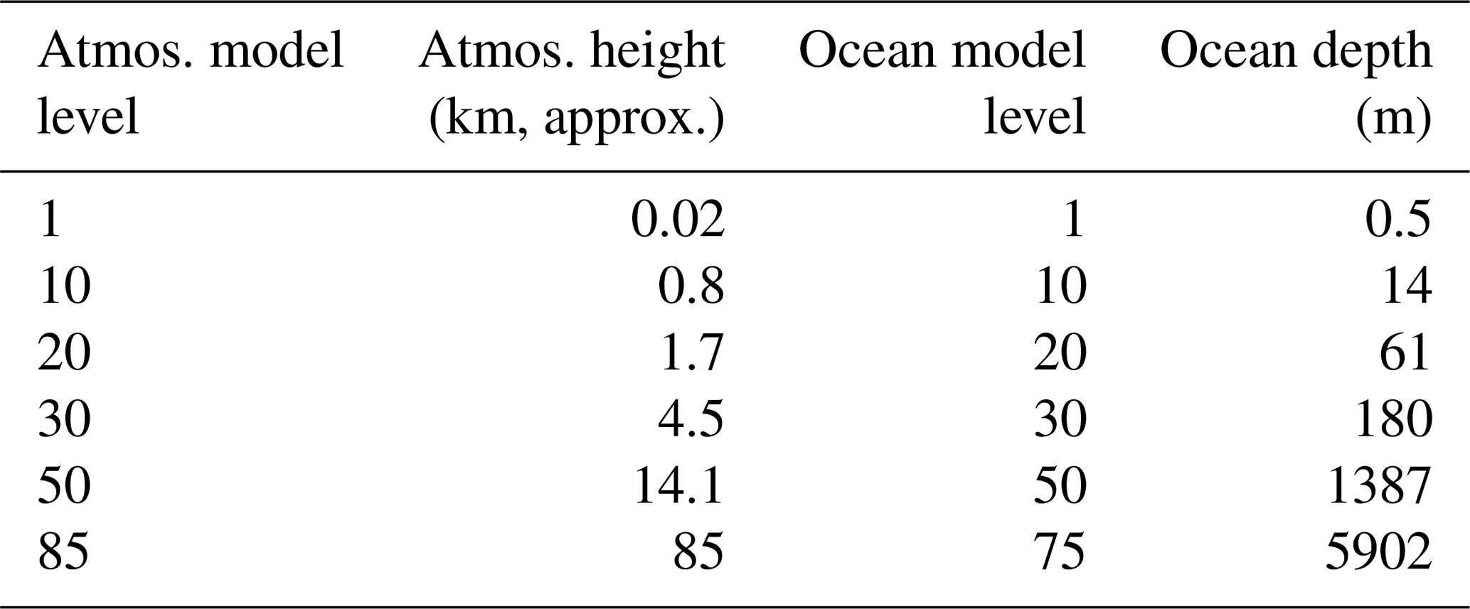
The configuration of the global coupled model HadGEM3-GC3.1 for submission to the CMIP6 DECK (Eyring et al., 2016) is described in Williams et al. (2017), Menary et al. (2018) and Kuhlbrodt et al. (2018). It incorporates a global atmosphere–land configuration called GA/GL7.1 (Walters et al., 2019), with a new modal aerosol scheme (GLOMAP mode; Mulcahy et al., 2018). The atmospheric model uses a regular latitude–longitude grid and has 85 levels extending to 85 km. The global ocean component is called GO6 (Storkey et al., 2018), which uses the Nucleus for European Modelling of the Ocean (NEMO) ocean model (Madec et al., 2017) at vn3.6, having a tripolar grid, with 75 ocean levels (and top level thickness of 1 m). The sea ice model configuration is GSI8.1 (Ridley et al., 2018), which uses the CICE5.1 model (Hunke et al., 2015). Coupling between atmosphere and ocean models is performed by the OASIS-MCT coupler (Valcke et al., 2015) with conservation for the heat and freshwater terms and with surface fluxes calculated on the atmosphere grid. The coupling period is set to 1 h for all models. A sample of the vertical resolution in atmosphere and ocean is shown in Table 1.
Table 1A selection of model levels in the atmosphere and ocean and their corresponding height/depth.
The HighResMIP protocol recommends the use of the MACv2-SP scheme (Stevens et al., 2017) for simplified and standardised aerosol forcing. This specifies the change of anthropogenic aerosol optical properties over time and hence enables easier comparison between different models, while retaining the model's own aerosol mean (non-varying) background natural climatology and hence requiring little or no additional tuning. It is used here in place of the prognostic GLOMAP-mode scheme, with model implementation described in Vidale et al. (2019a). Simulations representative of 1950 (spinup-1950, control-1950) use mean values over 1949–1958 of the time-varying dataset.
2.2 Model resolution differences
The different model resolutions used in this work, together with parameterisation and parameter choices, are summarised in Table 2. We will henceforth use the CMIP6 naming conventions and CMIP6 nominal resolutions when describing the models – this is calculated as a weighted mean of the diagonal distance across grid cells, binned into resolution categories. Henceforth, we use the terms “model resolution” and “model grid spacing” interchangeably, while Klaver et al. (2019) describe the effective model resolution based on kinetic energy spectra.
Table 2Parameter value changes between different model ocean (from top) and atmosphere (from bottom) resolutions, together with resolution naming conventions (in bold).
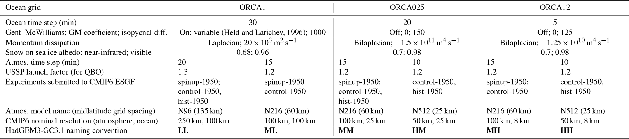
The HadGEM3-GC3.1 model has very few parameter values explicitly changed as model resolution is varied (Table 2). In the atmosphere, the only explicit parameter change is to the “USSP launch factor”, which is used to produce a reasonable period for the quasi-biennial oscillation (QBO) at different resolutions, as described in Walters et al. (2019). For the ocean model, there are more changes, principally because we move from a regime at 100 km resolution (LL model) where the ocean mesoscale (ocean eddies, boundary currents) are strongly tied to parameterisations and the requirements of numerical stability, to eddying regimes at 25 and 8 km where these properties are increasingly explicitly resolved. The parameter choices for the LL model are described in Kuhlbrodt et al. (2018), with key differences from 100 to 25 km resolution being the deactivation of the ocean eddy flux parameterisation (Gent and McWilliams, 1990) and the reduction of explicit dissipation parameters. The snow on sea ice albedo was adjusted to be lower in the LL model (by 2 %–3 %; see Table 2) due to excessive sea ice thickness particularly in the Arctic (Kuhlbrodt et al., 2018).
In addition to explicit parameter differences, some model parameters and schemes are self-tuning; that is, their controlling parameters vary automatically based on model resolution. These include the stochastic physics stochastic perturbation of tendencies (SPT) and stochastic kinetic energy backscatter (SKEB2) schemes, as described in Walters et al. (2019) and Sanchez et al. (2016).
Detailed descriptions of the atmospheric model differences, such as the impact of using MACv2-SP scheme, can be found in Vidale et al. (2019a), and further assessments of ocean model differences up to 8 km resolution are described in Storkey et al. (2018) and Mathiot et al. (2019).
2.3 CMIP6 HighResMIP forcing
The simulations described here follow the CMIP6 HighResMIP protocol (Haarsma et al., 2016) in terms of the forcing datasets used. The spinup-1950 and control-1950 experiments (Fig. 1) use mean values of the CMIP6 transient forcing datasets for aerosol (as above), solar (Matthes et al., 2017), ozone concentration (Hegglin et al., 2016) and greenhouse gas (GHG) forcings (Meinshausen and Vogel, 2016). Aerosol uses a monthly mean from the 1950–1959 period; ozone and solar use a monthly mean over 22 years centred about 1950 (in order to mean over the 11-year solar cycle); GHG uses the 1950 value of GHG global concentrations. The hist-1950 simulations (not analysed here) use the time-varying versions of these forcings.

Figure 1The HighResMIP experimental design, including the names of the component experiments and an indication of their relationship.
2.4 Computational characteristics
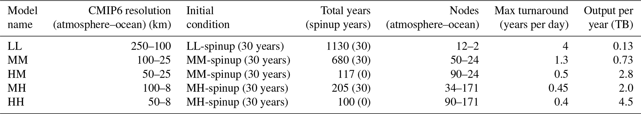
Details of the computational performance of the models at different resolutions can be found in Vidale et al. (2019b). Table 3 shows an overview of the total run lengths, initial conditions for each simulation, model costs and the volume of data output, primarily of the raw priority 1 diagnostics for the HighResMIP data request (Juckes et al., 2019). Since we expect the higher-resolution models to represent weather processes and events in an improved way, there is a requirement for more high-frequency output (1-, 3-, 6-hourly on multiple atmospheric levels, as well as daily ocean surface output) in order for us to assess these processes.
Table 3For each model resolution for the control-1950 simulation: the nominal CMIP6 resolution, the initial condition, total simulated years and costs of various model resolutions on a Cray XC40 with 36 cores per node, together with raw model output volumes.
2.5 Model simulations
Most of the model data used in the following analysis are available from the CMIP6 Earth System Grid Federation and can be located using the information in M. Roberts (2018, 2017a, b, c, d) for LL, MM, HM, MH and HH resolutions, respectively. Other model resolutions are not part of the official HadGEM3-GC3.1 CMIP6 HighResMIP submission, with the data available on request.
The analysis in this work uses data from the spinup-1950 and control-1950 HighResMIP experiments and hence is a representation of 1950 climatological conditions. It should be noted, when comparing these data to observations, that globally complete observational data are typically only available post-1970s, and hence one expects that some component of any “bias” will be attributable to this difference in the simulation and observational periods.
2.5.1 The spinup-1950 protocol
Given the expense of the higher-resolution models, the typical spinup procedure as used in CMIP6 DECK simulations (many hundreds of years of pre-industrial (PI) spinup before piControl and historic simulations are initialised; Eyring et al., 2016) is simply not feasible here. Hence, the HighResMIP protocol recommends 30–50 years using the spinup-1950 protocol from specified ocean and atmosphere initial conditions; here, we use 30 years. This “spun up” state is then used to initialise the control-1950 and hist-1950 simulations as illustrated in Fig. 1.
The common initial conditions for the ocean temperature and salinity are derived from the January 1950–1954 mean of the EN4 ocean analysis (Good et al., 2013). This is bilinearly interpolated to the model ocean grid. For the higher ocean resolutions (25 and 8 km), it was found that several days of simulation with a very short ocean time step (typically one quarter of the standard value) were needed in order to remove small-scale instabilities introduced by the interpolation, particularly in the high Arctic and where the Mediterranean and Black seas meet. The model was then restarted at 1 January 1950 with these derived ocean and sea ice initial conditions.
The atmosphere initial condition is derived from ERA-20C (Poli et al., 2016) in January 1950. Initial conditions for sea ice are taken from previous ocean–sea ice simulations (at the same resolution) valid around 1979, since methods to initialise different sea ice models with common variables are less well developed and with the assumption that sea ice has a timescale of only several decades to quasi-equilibrate. The soil moisture has a relatively long memory, and its initial condition was taken from a previous HighResMIP atmosphere-only simulation using the same atmosphere resolution.
The spinup-1950 experiment with models using 25 and 8 km ocean resolutions were only performed with one atmosphere resolution – MM and MH, respectively – both using the 100 km atmosphere.
2.5.2 The control-1950 protocol
The final states of all the model components at the end of spinup-1950 simulation are used to initialise both the control-1950 and hist-1950 experiments. As noted above, the MM spinup-1950 is used as initial condition of both MM and HM, and the MH spinup-1950 was used for both MH and HH. This method seemed to work well for the ocean component, but for the soil moisture in the land component it was found that the more inhomogeneous soil properties at 50 km (HM, HH) resolution tended to retain less water. This led to a pulse of freshwater from land to ocean at the start of the control-1950 and hist-1950 simulations. To prevent this, the soil moisture from a previous 50 km simulation was inserted into initial conditions for the HM and HH simulations.
The control-1950 experiment is required to be at least 100 years in length but can be much longer – it is the HighResMIP equivalent to the CMIP6 piControl. It uses the same forcings as spinup-1950. In this work, there are 1000 years of LL, 600 years of MM and 150 years of MH available for analysis.
2.5.3 The hist-1950 protocol
These simulations have the same initial conditions as their respective control-1950 models. The forcings are now the time-varying CMIP6 forcings. Since we recognise that the models will continue to drift over time, due to the short spinup, we can use the difference between the hist-1950 and control-1950 simulations as an estimate of the impact of changing forcings on the climate state, assuming a common drift between the two simulation types. Analysis of these simulations is outside the scope of this work.
3.1 Initial spinup and radiative balance
The radiative balance of the different resolution models is shown in Fig. 2, in terms of the top-of-atmosphere (TOA) radiation, its outgoing shortwave and longwave (OSR, OLR) components, and the global mean surface temperature (ST), together with observational estimates where possible. The TOA starts at between −1.5 and −1 W m−2 in the initial state of the models, and by the end of 30 years, they have all adjusted to within ±0.3 W m−2, compared to an estimate of observed TOA in the range 0.23–0.6 W m−2 during 1985–2010 (Stephens et al., 2012; Wild et al., 2013; Allan et al., 2014). The mean TOA over the control-1950 period for each model is indicated by the box-and-whisker plot to the right of Fig. 2. This radiative adjustment is accomplished in different ways by the different resolution models. The LL model has the largest changes in radiative terms with a sharply increasing OSR by nearly 2 W m−2 over the initial 30 years (Fig. 2b), together with a reduction of 3.5 W m−2 in the OLR (Fig. 2c), both of which are deviations from the observed values. The latter is consistent with a 2 K decrease in the ST (Fig. 2d), while the former is consistent with an increase in Arctic sea ice area (Fig. 5). During the control-1950 simulation, the surface temperature warms (Fig. 2d) and the OSR and OLR continue to adjust gradually over several hundred years.
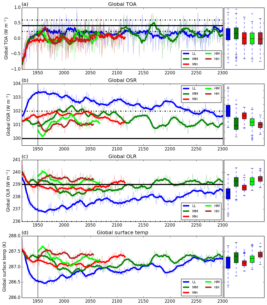
Figure 2Time series of globally averaged quantities for three ocean resolution spinup-1950 simulations (x-axis nominal years: 1920–1950 here) and five control-1950 simulations initialised from these conditions (x-axis nominal years: 1950–2300). (a) Top-of-atmosphere (TOA) radiation, W m−2; (b) outgoing shortwave radiation (OSR), W m−2; (c) outgoing longwave radiation (OLR), W m−2; (d) surface temperature, K. The horizontal black lines are estimates (solid) and uncertainty (dashed) of fluxes from Wild et al. (2013).
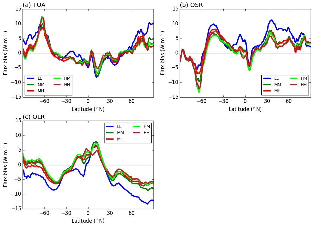
Figure 3Annual mean zonal mean model radiation biases (years 50–100) of top-of-atmosphere radiation components against CERES-EBAF observations for 2000–2018 (Kato et al., 2013). (a) Top-of-atmosphere net radiation; (b) outgoing shortwave radiation; (c) outgoing longwave radiation.
For comparison, as shown in Vidale et al. (2019a), the atmosphere-only simulations have a TOA which starts at around −1.5 W m−2 in 1950, with surface temperature of 288 K, OSR around 100–101 W m−2 and OLR around 240.5–241.5 W m−2 (which adjusts to around 239.5–240.5 W m−2 at 1980 when the TOA is closer to zero).
The adjustments of the MM and MH models are similar, and they stay closer to the observational estimates. Here, the OSR increases by 0.5–1 W m−2 at the start of the control-1950 (after small changes in the spinup-1950 period), while the OLR reduces by up to 2 W m−2 (partly in the spinup-1950 and partly in the control-1950 periods) again consistent with a surface temperature drop of about 0.75 K. The MM model continues to adjust for the first 40 years of control-1950, with reducing ST, before settling into a quasi-equilibrium with global TOA of +0.1–0.2 W m−2 and increasing ST. The MH model only cools very slightly during the control-1950 simulation from its initial conditions and is the model that has the smallest trends over the control-1950 period and the smallest deviation globally from the initial conditions in all of the time series. In terms of robustness, the ML and LM models (not shown) broadly follow their ocean resolution equivalents (LL and MM, respectively).

Figure 4Annual mean model bias over years 50–100 in cloud radiative forcing (W m−2) for (a, c, e) shortwave cloud forcing and (b, d, f) longwave cloud forcing, compared to CERES-EBAF observations for 2000–2018 (Kato et al., 2013).
The oscillations in the MM TOA after 100 years are relatively large and relate to Antarctic sea ice variability and particularly to a large polynya that opens and closes over time in the Weddell Sea. This is a relatively common feature among climate model simulations (Griffies et al., 2015; Dufour et al., 2017; Cabré et al., 2017).
The models have not been tuned (beyond the shared, common scientific configuration developed for the HadGEM3-GC3.1 CMIP6 DECK model) for a specific long-term TOA radiation, so it is either chance or some inherent property of this coupled system that enables all models to achieve a relatively small net TOA balance over such a short time. For comparison, the equivalent HadGEM3-GC3.1 DECK pre-industrial control (piControl) simulations have mean TOA of 0.2 and 0.31 W m−2 over several hundred years (LL and MM resolutions after 652 and 353 years of spinup, respectively; Menary et al., 2018).
The zonal mean TOA, OSR and OLR biases compared to the Clouds and the Earth's Radiant Energy System Energy Balanced and Filled product surface fluxes edition 4.0 (CERES-EBAF; Kato et al., 2013) are shown in Fig. 3. This confirms that the largest differences occur when the resolution is changed from LL to any other resolution. At low and midlatitudes, the TOA bias is relatively small, but this is due to a compensation between OSR and OLR components, with OLR biased negative at nearly all latitudes and OSR biased positive. All models have positive OSR biases at midlatitudes apart from near Antarctica where there is a negative bias.
The spatial patterns of cloud radiative forcing (CRF) biases against CERES-EBAF (Kato et al., 2013) are shown in Fig. 4 for both shortwave and longwave components (SW, LW). The large-scale patterns of bias are consistent across model resolutions, but there are significant regional differences. As we increase the resolution, for the Atlantic basin, there are reductions in the SW CRF bias in both the tropics and over the Gulf Stream–North Atlantic Current, in the stratocumulus/upwelling regions (off the west coasts of South America, South Africa and to a lesser extent North America) and in the western Pacific. In contrast, there is an increase in bias in the eastern tropical Indian Ocean and over South America. For the LW CRF, there is less change: the bias in the tropical Atlantic changes from a negative bias to the south of the Equator to a positive bias to the north, which links to the precipitation biases shown later. A negative bias also increases with increased resolution in the eastern Indian Ocean (perhaps somewhat compensating for the SW CRF bias).
The time series of sea ice area in the Arctic and Antarctic for March and September (approximately the extremes of the respective seasonal cycles) are shown in Fig. 5, together with some observational estimates (HadISST1.2, Rayner et al., 2003; HadISST.2.2.0.0, Titchner and Rayner 2014), noting that the observations are representative of years 1990–2009, while the model is simulating the year 1950. As noted previously, the LL model has a large increase in Arctic sea ice area over the initial decades before approaching the climatology of the other models. All models have somewhat more Arctic sea ice in both summer and winter than observations. In the Antarctic winter, the MM model displays considerable decadal variability (particularly later in the simulation, as noted in the TOA variability previously) which is not so evident at other resolutions and is due to a large polynya opening and closing in the Weddell Sea. Summer Antarctic sea ice values are improved over previous versions of the model, particularly at MM resolution for which large-scale warming of the Southern Ocean has been a persistent model bias. This has been achieved primarily from reduced atmospheric flux biases (Bodas-Salcedo et al., 2016; Hyder et al., 2018; Williams et al., 2017), though a warm bias does still remain (see Fig. 7).
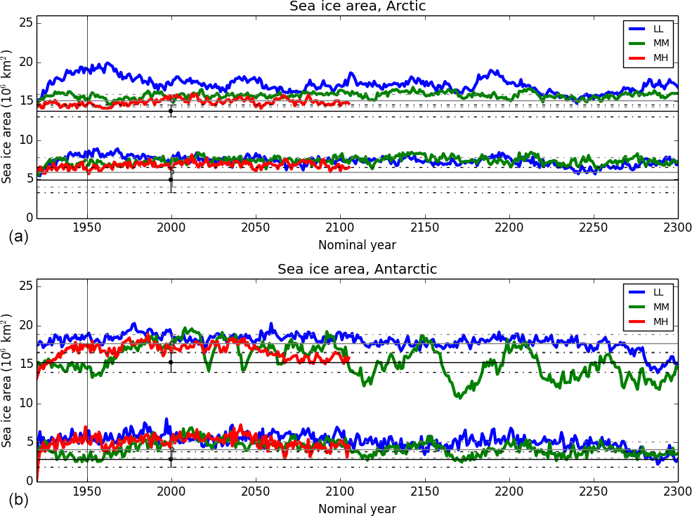
Figure 5Time series of sea ice areas in the (a) Northern Hemisphere and (b) Southern Hemisphere for three model resolutions, for spinup-1950 and control-1950 simulations. In each hemisphere, the winter and summer months (March, September in NH; September, March in SH) are shown by the upper and lower groups of contours, respectively. Observations are HadISST1.2 (black line) and HadISST.2.2 (gray line), with their mean value over 1990–2009, are shown as the solid line and the maximum and minimum during that period as dashed lines.
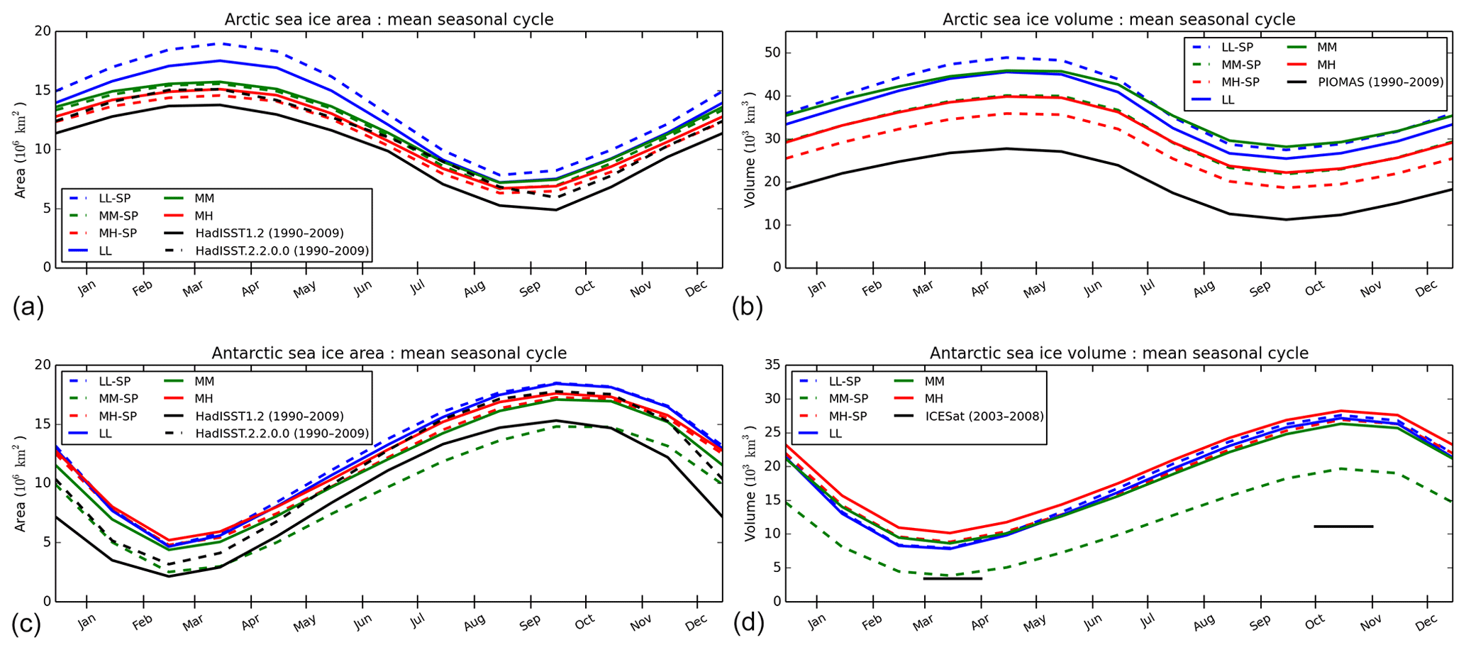
Figure 6Seasonal cycles for (a, c) sea ice area and (b, d) sea ice volume from models and observations, in the (a, b) Arctic and (c, d) Antarctic regions. The dashed and solid colours refer to different model periods (dashed is the 10-year mean at the end of spinup-1950; solid is the 20-year mean at the end of control-1950). Observed sea ice area is from HadISST1.2 (1990–2009) and HadISST2.2.0.0 (1990–2009), and sea ice volume is from the Pan-Arctic Ice Ocean Modeling and Assimilation System (PIOMAS) model (1990–2009) and ICESat (2003–2008).
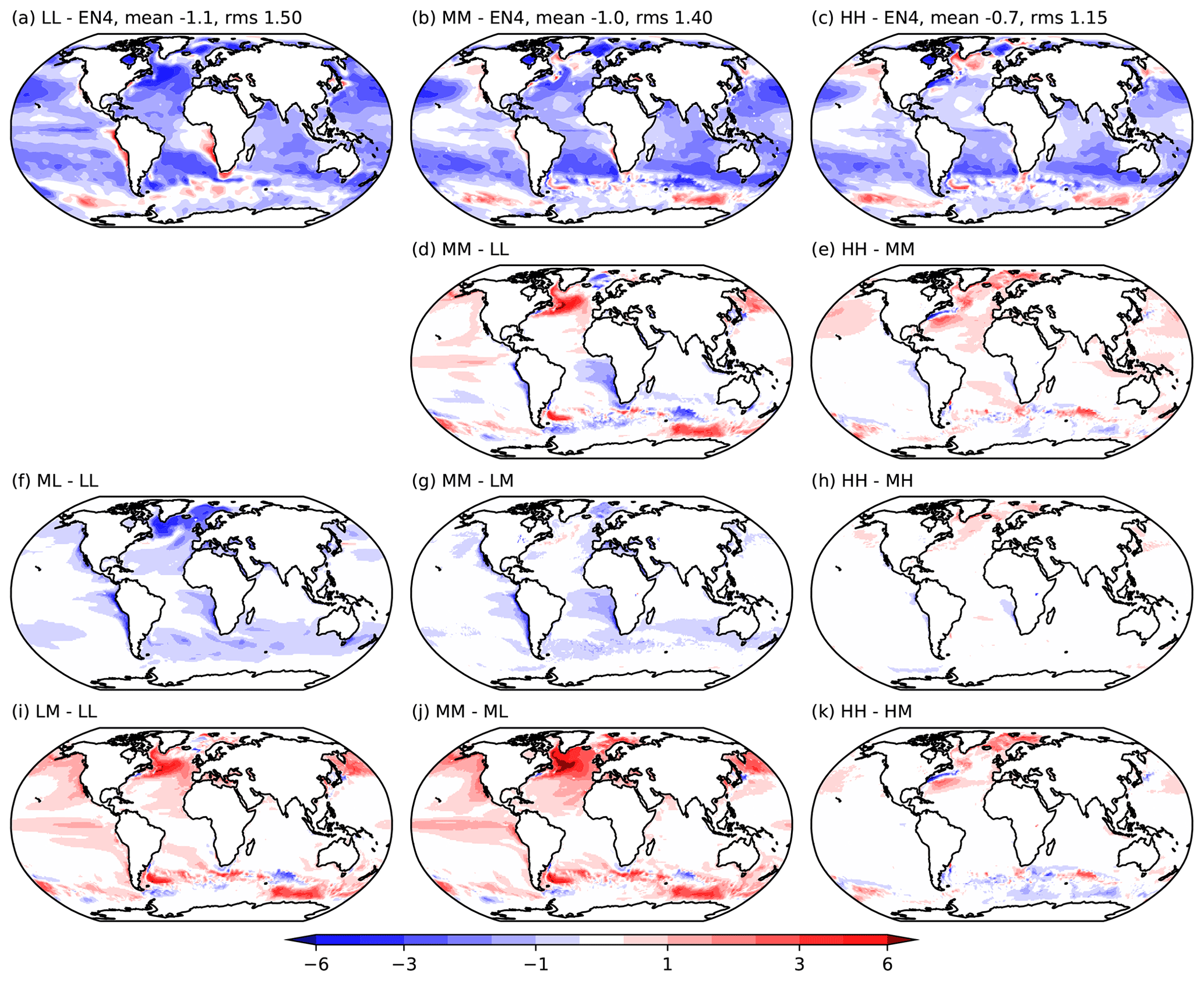
Figure 7Top row: model SST bias in control-1950 years 50–100 vs. EN4 (1950–1954 mean), with the mean and rms bias shown; second row: the total SST differences between MM-LL and HH-MM resolutions; third row: the impact of changing the atmosphere resolution at each reference ocean resolution; bottom row: the impact of changing the ocean resolution at each reference atmosphere resolution. Units are K. Points that contain annual mean sea ice are masked.
The sea ice area and volume seasonal cycles are shown in Fig. 6 at the end of both the spinup-1950 and control-1950 simulations. There are few observational means to assess sea ice volume, and so here we use the Pan-Arctic Ice Ocean Modelling and Assimilation System sea ice reanalysis (PIOMAS; Zhang and Rothrock, 2003; Schweiger et al., 2011) model as a reference in the Arctic (1990–2009) and satellite estimates from ICESat (Ice, Cloud, and land Elevation Satellite) for the Antarctic during 2003–2008 (Kurtz and Markus, 2012). PIOMAS has been shown to compare well with ICESat thickness for the periods where ICESat is present (Schweiger et al., 2011), and this gives us confidence to use the data throughout the year and over the longer evaluation period (1990–2009). The seasonal cycle amplitude and phase of sea ice area are well captured in the models except for LL in the Arctic, which has too much sea ice. All the models have more sea ice volume than is indicated by the PIOMAS model and ICESat in the Arctic and Antarctic, respectively. In the Arctic, the volume increases over time in the MM and MH simulations while reducing somewhat in LL, while in the Antarctic the MM volume starts lower than the other models but adjusts to a similar mean state.
3.2 SST adjustment and biases
The SST biases at the end of the control-1950 period (averaged over years 50–100) are shown in Fig. 7 for each model resolution. These are shown both as model bias compared to initial condition (top row) and as inter-resolution differences for the total change (due to atmosphere plus ocean resolution), change due to atmosphere resolution alone, and change due to ocean resolution alone (rows two, three and four, respectively). A common feature across the models is a generally cold midlatitude bias, which may partly reflect the experimental design of using EN4 1950–1954 initial conditions, the short spinup-1950 period, the constant 1950s forcing derived from CMIP6 and a consequently negative TOA in the first few decades (Fig. 2a) but is also a feature found in many climate models and experiments (see Flato et al., 2013, Fig. 9.13; Kuhlbrodt et al., 2018).
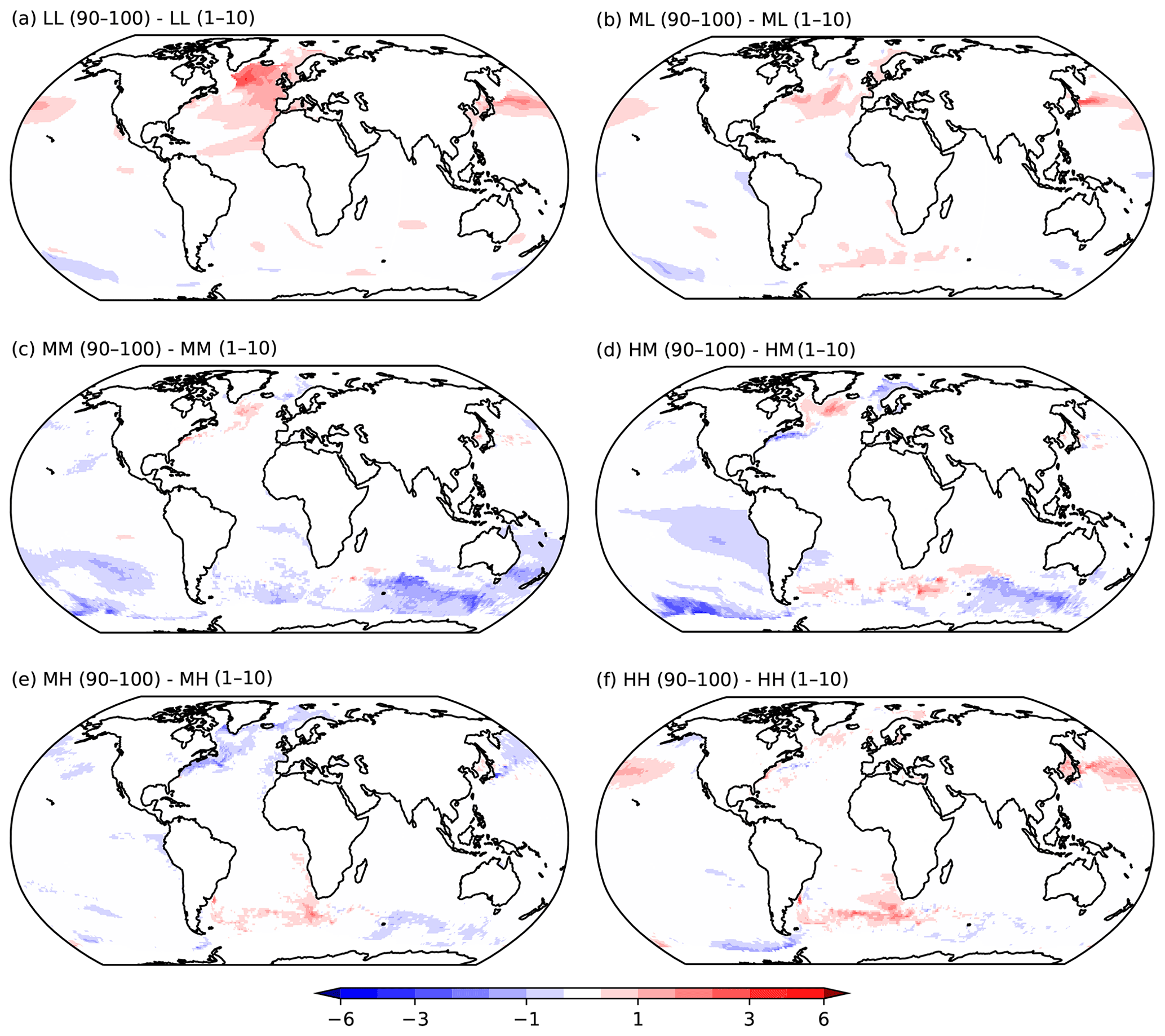
Figure 8The change in SST over 100 years of the control-1950 simulation illustrated by the difference between years 90–100 and years 1–10.
The biases typical for a 100 km ocean model (Danabasoglu et al., 2014) are evident in Fig. 7a for LL and also described in Kuhlbrodt et al. (2018). They are strongest over the boundary currents in the North Atlantic and northwest Pacific, with cold biases of more than 5 K, and over the tropics with a cold bias of 1–2 K. Warm biases over the stratocumulus decks to the west of southern Africa, South America and California are also evident, as well as warm biases in the regions where boundary currents separate from the coastline (particularly the Gulf Stream and Kuroshio). Comparing this to the 25 km model (MM, Fig. 7b, d), there are large reductions in both boundary current and tropical biases, and some reductions in the warm stratocumulus biases and the warm bias at the Kuroshio separation. These come at the expense of an enhanced warm bias in the Southern Ocean, which is also common in models at this resolution (Bodas-Salcedo et al., 2014; Flato et al., 2013, Fig. 9.2b), and is due to errors in the atmospheric fluxes (Bodas-Salcedo et al., 2014; Hyder et al., 2018) and due to the intermediate regime in the Southern Ocean in which the ocean models have no eddy parameterisation but also a poor explicit representation of eddies (Hallberg, 2013; Moreton et al., 2019). Although still sizable, the bias has been considerably reduced compared to previous versions of the model (Williams et al., 2017).
Comparing the 8 and 25 km ocean models (HH and MM; Fig. 7e), there is further warming in the Atlantic in the eddy-rich model with mixed results compared to the bias and some further cooling in the stratocumulus regions, and over the Gulf Stream separation the bias switches from warm to cold. The Southern Ocean warm bias is slightly reduced compared to MM but remains larger than the LL bias.
There is no clean way to attribute the biases to either atmosphere or ocean resolution due to complex coupled interactions, but rows 3–4 of Fig. 7 show the impact of atmosphere and ocean resolution change only, respectively, for a given resolution of the other component. The largest changes are found between the L and M resolution components, with smaller changes at higher resolutions (consistent with C. D. Roberts et al., 2018). For the L and M resolution ocean, a higher-resolution atmosphere tends to produce a cooler ocean SST, particularly in the ocean upwelling regions (as also seen in Gent et al., 2010 and Small et al., 2014, 2015), the Southern Ocean and the North Atlantic. A higher ocean resolution, meanwhile, tends to produce a warmer SST particularly in boundary currents and other high gradient regions, with changes over 6 K (Griffies et al., 2015; Small et al., 2019). Differences between HH and MH, HM are relatively smaller, though the improved separation of the Gulf Stream from the North American coast and consequent reduction in warm bias is evident in the dipole of SST change with the eddy-rich ocean (Fig. 7k) as also seen in Small et al. (2019).
To contrast the biases above to model surface drift, and hence the effectiveness of the short spinup in the experimental design, Fig. 8 shows the SST differences between the start and end of the control-1950 simulation. The different model resolutions evolve in distinct ways. LL and ML (Fig. 8a, b) both warm in the northern Pacific and Atlantic basins, the latter consistent with the reduced Arctic sea ice as seen earlier and an increasing AMOC and northward heat transport (see later). MM and HM (Fig. 8c, d) both cool at high latitudes in the Southern Hemisphere and warm slightly in the northern North Atlantic; the HM model has some additional cooling in the southeast Pacific, likely associated with reduced coastal warm bias. MH and HH (Fig. 8e, f) both have a slight warming in the South Atlantic near the Antarctic Circumpolar Current. However, it is clear that the magnitude of this drift is considerably smaller than the mean bias shown in Fig. 7, such that the bias plot at the end of spinup-1950 (not shown) is little different from Fig. 7. The only notable region with similar magnitude of drift and bias is the LL North Atlantic warming and part of the Southern Ocean cooling in MM and HM.
The annual mean 2 m temperature biases over land are shown in Fig. 9 using model means over years 50–100, compared to the Climate Research Unit time series 4.01 dataset for period of 1940–1960 (CRU TS; Harris et al., 2014). The warmer SSTs and reduced sea ice extent in the Arctic Ocean between LL and the higher-resolution models give significantly warmer surface temperatures over Scandinavia, northern Russia and Alaska of 2–3 K. Tropical cold biases are also reduced as resolution is increased, leading to the HH model having a considerably smaller global root mean square (rms) bias.
The results above indicate that, for the surface climatology, the HighResMIP simulations are adequately long to illustrate robust differences due to model resolution. However, the deeper ocean requires much longer to come into any pseudo-equilibrium, and these drifts are described next.
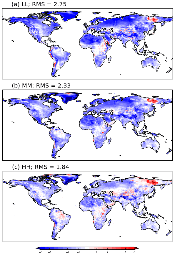
Figure 9Annual mean bias in 2 m temperature over land (∘C) for control-1950 simulations (years 50–100) relative to CRU TS (Harris et al., 2014) for the period of 1940–1960.
3.3 Deep ocean evolution
The evolution of subsurface ocean changes from the initial state (henceforth referred to as ocean drift) at different model resolutions is shown in Figs. 10 and 11 for temperature and salinity, respectively, for both the global ocean (left column) and the Atlantic basin (40∘ S–70∘ N excluding the Mediterranean, right column), for all model resolutions with a spinup-1950 simulation. For the global ocean, the temperature and salinity drifts differ mainly in their magnitude, while the Atlantic drifts have different patterns. These drifts may be compared to those in Small et al. (2014), Griffies et al. (2015) and Kuhlbrodt et al. (2018).

Figure 10The mean ocean potential temperature anomaly (compared to year 1) on model levels against time for the (left) global and (right) Atlantic Ocean basins, from the spinup-1950 period to the first 210 years (where available) of control-1950. Note the different scales for the different regions.
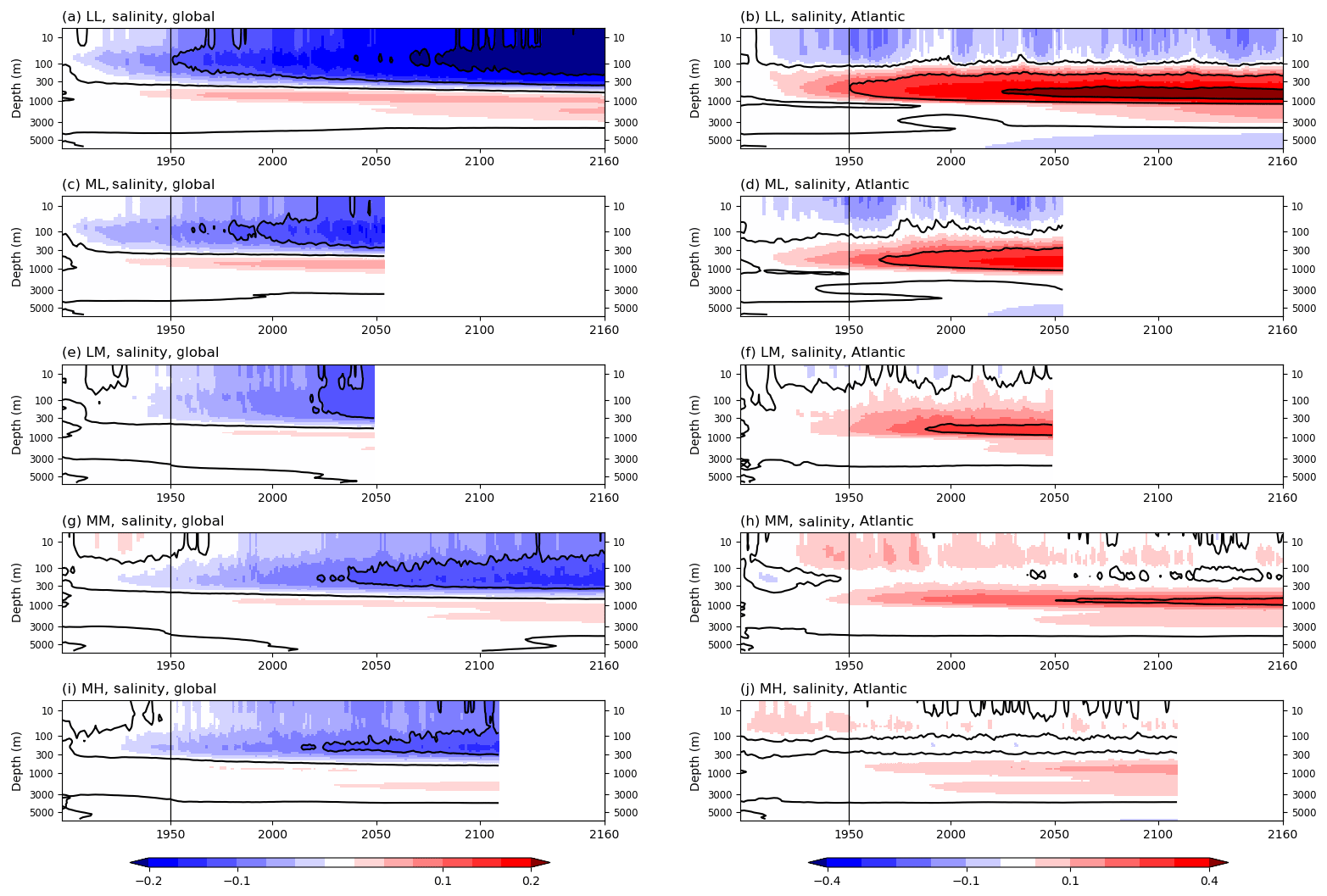
Figure 11As Fig. 10 but for ocean salinity, again with different scales on the left and right.
All models have a global cooling of 0.5–1 K over the top 200 m (Fig. 10, left column) which gradually reduces over time and a warming centred at 800 m, with an enhanced magnitude in the L ocean models. The LM and MM models have a deep warming not seen in other models, which is likely associated with the Southern Ocean bias (not shown). The global salinity drift (Fig. 11, left column) shows all models have a freshening over the top 300 m with magnitude increasing over time. They also have an increase in salinity between 1000 and 2000 m, which is larger with the L ocean.
The temperature evolution in the Atlantic (Fig. 10, right column) is similar to the global drift, with near-surface cooling and a warming at mid-depths, both of which are stronger in the L ocean. The warming at mid-depths is also associated with an increase in salinity (Fig. 11, right column), which is also seen in Griffies et al. (2015) and Kuhlbrodt et al. (2018), and is likely to be associated with the AMOC circulation, production of North Atlantic Deep Water (NADW) and biases in representing deep overflows in the North Atlantic (Danabasoglu et al., 2014). The change from L to a higher-resolution ocean causes the surface Atlantic salinity bias to switch from a freshening to a positive increase, with the eddy-rich MH resolution notable for having greatly reduced salinity drifts in the Atlantic – these differences are consistent with differences in (tropical) precipitation as shown later.
Figure 10c–d and e–f illustrate the impact of atmosphere and ocean resolution on these drifts. Using a higher-resolution atmosphere in ML (Fig. 10d) suggests a reduction in the Atlantic mid-depth warming (perhaps an improvement in the NADW), while LM (Fig. 10e, f) shows a slight reduction in the magnitude of warming at 1000 m and the warming of the bottom waters globally associated with the Southern Ocean bias.
Given the experimental design, it is difficult to disentangle drifts due to imbalances in surface forcing from processes that may be poorly represented. As discussed in Griffies et al. (2015), von Storch et al. (2016) and Small et al. (2019), the evolution of the subsurface ocean depends on fluxes of heat (and salt) from either parameterised or explicitly represented processes (e.g. vertical diffusion, advective fluxes from mean, mesoscale and submesoscale circulation). The changes in the subsurface ocean over time with resolution shown here are consistent with these previous studies, which would indicate an important role for upward heat transport from vertical mesoscale fluxes. The models shown here do not contain a submesoscale eddy parameterisation, which may be important to represent unresolved processes (Fox-Kemper et al., 2011), but they do have enhanced ocean vertical resolution in the near surface (Table 1) compared to the models referenced above, which may also be important.
The information above has shown that 100 years is insufficient to saturate the deep ocean drifts, as would be expected. However, some differences with resolution do seem to be robust and possibly linked to process improvement, particularly in the Southern Ocean where the eddy-rich MH simulation greatly reduces the deep warm temperature drift and in the North Atlantic for both temperature and salinity.
The spatial patterns of the temperature and salinity biases at 950 m depth are shown in Fig. 12 for LL, MM and HH, as a mean over years 50–100, compared to EN4 1950–1954. As indicated in the previous figures, the LL model has warming and increased salinity over much of the Atlantic with an enhancement in the western tropical Atlantic. There biases are mostly reduced in MM and HH simulations, where the main bias switches to the eastern North Atlantic with potentially some role for the Mediterranean outflow. In the region of the Gulf Stream separation from the North American coast, the HH model has a cold and slightly fresh bias opposite to the lower resolutions. Over the rest of the global oceans, the LL model has warming and increase in salinity at mid–high latitudes in the Pacific Ocean which is somewhat reduced in HH, while all the resolutions have cooling and freshening in the northwest Indian Ocean and warming in the southwest Indian Ocean.

Figure 12Biases at 950 m depth at different model resolutions for (a, c, e) temperature and (b, d, f) salinity (model years 50–100 minus the EN4 mean for 1950–1954).
The eddy-rich ocean simulation, MH, has both the minimum in surface adjustment (of radiation and temperature) as well as the smallest deep ocean drifts from the EN4 initial conditions. It is unclear whether this is due only to improved representation of key processes (for example, in the Southern Ocean and Atlantic), or whether by chance it is better able to adjust from these initial conditions. It should also be noted that interior biases can be exacerbated by spurious mixing, especially in the 1∕4∘ ocean model (Griffies et al., 2000; Ilicak et al., 2012; Megann, 2018). The improvements show some similarity to those in Griffies et al. (2015), and hence a multi-model study using the HighResMIP experimental design is needed to firmly establish whether such an increase in ocean resolution can robustly reduce deep ocean drifts and hence establish whether higher-resolution (ocean/coupled) models require less spinup time; this work is ongoing as part of PRIMAVERA.
3.4 Mean state precipitation biases
Changes in the annual mean precipitation bias against Global Precipitation Climatology Project (GPCP) version 2.3 1979–2014 (Adler et al., 2018) with resolution are shown in Fig. 13, averaged over model years 50–100 of control-1950, and are generally consistent with those found in the multi-model analysis of Vannière et al. (2018). The mean biases are shown in the top row, together with the total differences (atmosphere plus ocean resolution changes, row two), and then the impact of atmosphere and ocean resolution changes individually (rows three and four, respectively).
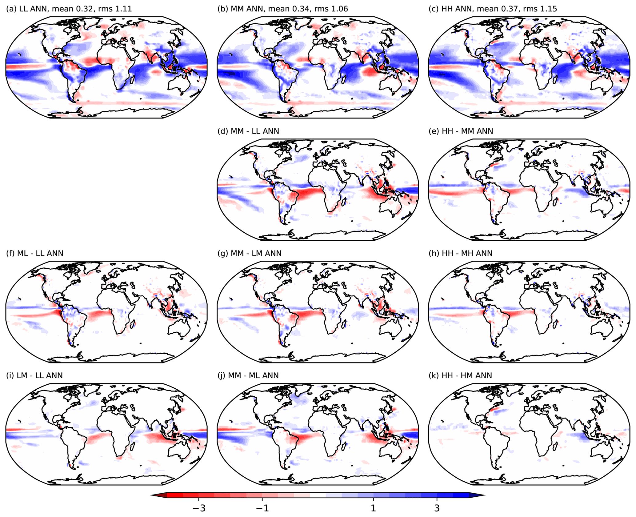
Figure 13Top row: annual mean model precipitation bias of control-1950 model years 50–100 vs. GPCP_v2.3 1979-2014; second row: the total precipitation differences between MM-LL and HH-MM resolutions; third row: the impact of changing the atmosphere resolution at each reference ocean resolution; bottom row: the impact of changing the ocean resolution at each reference atmosphere resolution. Units are mm d−1.
Some aspects of the large-scale biases are common across all resolutions, consistent with those shown in Williams et al. (2017). There is excessive precipitation in the western tropical Pacific, southeast Asia, the western Indian Ocean and the South Pacific Convergence Zone (SPCZ), which also includes a double Intertropical Convergence Zone (ITCZ) error in the east Pacific (Lin, 2007).
In the tropical Atlantic, there is a dipole error of 2–3 mm d−1 across the Equator in LL with too much precipitation in the south and too little in the north, with significant consequences for land precipitation over South America. This error is markedly reduced in the MM model (Fig. 13d) and further reduced to the south of the Equator in HH (Fig. 13e), together with a reduction in the dry bias over west Africa (Fig. 13d). Richter et al. (2012) attribute part of this bias to wind stress and consequent ocean temperature errors, and indeed Fig. 7g does indicate significant reductions in the SST warm bias in the Atlantic. In the Pacific, the LL model has a double ITCZ error which reaches the eastern Pacific coastline, which is reduced at higher resolutions at the expense of further increases in excessive precipitation both to the north and south of the Equator. There is a reduction in the dry bias on the Equator in the Pacific at higher resolutions and some improvement over the Maritime Continent and India (Fig. 13d, e), with an increased dry bias in the eastern Indian Ocean. The subpolar North Atlantic has increased precipitation at higher resolutions, primarily due to the ocean and likely associated with a warmer SST.
Atmosphere and ocean resolutions both play an important role in these changes (Figs. 13f, g, h and 12i, j, k, respectively), with a higher-resolution atmosphere tending to be dry to the south of the Equator and wet to the north with a similar magnitude at each ocean resolution, while the ocean resolution change is much bigger between L and M apart from over the Gulf Stream.
The change in tropical Atlantic precipitation is consistent with an ITCZ located further north at higher resolution. This would be consistent with increased AMOC at higher resolution causing SST gradient changes (Jackson et al., 2015; also Fig. 7d, e) and may also be a consequence of a change in the global energy budget leading to shifts in the Hadley cell/ITCZ position (Bischoff and Schneider, 2016). The precipitation and consequent evaporation changes in the tropical Atlantic are also consistent with the salinity drifts shown in Fig. 11.
3.5 Atlantic Ocean meridional circulation and transport
The Atlantic northward heat transport (NHT) and Atlantic meridional overturning circulation (AMOC) time series are shown in Fig. 14 at 26.5∘ N and are calculated in a consistent way to observations for the RAPID-MOCHA array for 2004–2017 (Smeed et al., 2017; Johns et al., 2011) using the RapidMoc algorithm described in Roberts et al. (2013) and Roberts (2017). The MM and MH models increase both NHT and AMOC over the 30-year spinup-1950 period and subsequently vary about this mean state with no significant further drift evident. The LL model has decreasing transport over the spinup-1950 period (Fig. 14b), but over the 100-year control-1950 period both AMOC and NHT gradually strengthen to a state which is then maintained stably for many hundreds of years. This state is such that the AMOC strength is similar to MM, but the NHT remains about 10 % lower. This evolution is consistent with the SST drift discussed above, with increasing AMOC and NHT gradually warming the North Atlantic.
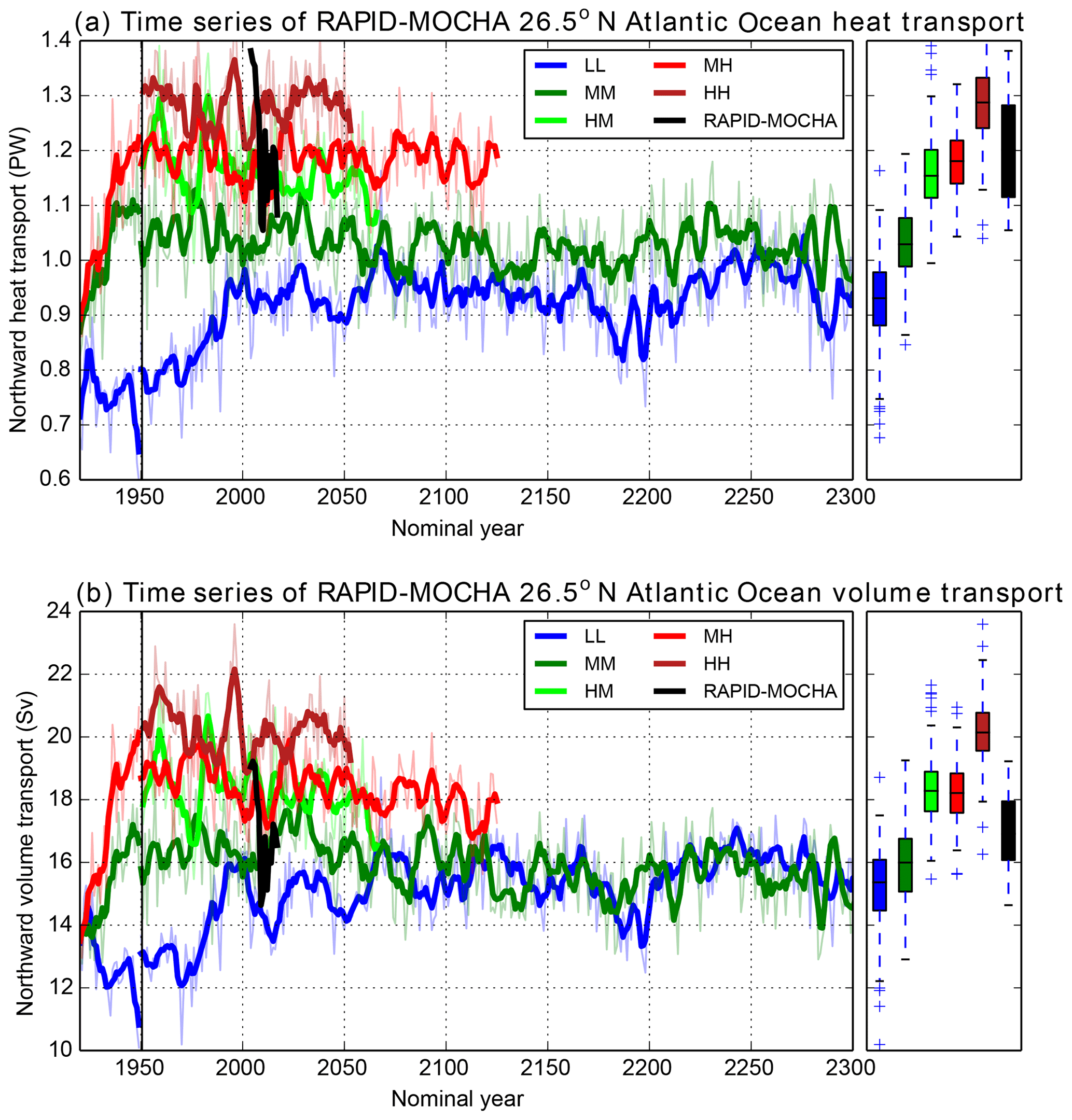
Figure 14(a) Time series of annual mean (January–December) Atlantic northward ocean heat transport at 26.5∘ N calculated consistently with the RAPID-MOCHA array using the RapidMoc code (C. D. Roberts, 2017). (b) As above but for volume transport, i.e. the Atlantic meridional overturning circulation at 26.5∘ N and 1000 m depth, with net transport across sections subtracted. Different model resolutions over the spinup-1950 and control-1950 simulations are shown together with the RAPID-MOCHA observations in black. The thick line shows a 5-year running mean of the annual values (thinner lines). A box-and-whisker plot on the right (using the control-1950 data) shows the lower to upper quartile range as the coloured box; the median (black line within that box) and the whiskers show the range of the data (excluding flier points shown by the + symbol).
The MH and HH models have NHT (Fig. 14a) which is most consistent with the observations, suggesting an important role for an eddy-rich ocean improving boundary current representation (Treguier et al., 2012; Roberts et al., 2016). However, for AMOC transport, the observations are perhaps more consistent with the lower-resolution models. This apparent inconsistency has been investigated previously by Msadek et al. (2013) and C. D. Roberts et al. (2018). Using a breakdown of heat transport components from the RAPID-MOCHA array (Smeed et al., 2017; Johns et al., 2011), they showed that the amount of NHT was typically underestimated due to both a too-weak AMOC and too little heat transport per Sverdrup of AMOC strength. The same breakdown for the model resolutions is shown in Fig. 15 as well as the AMOC profile with depth. All the models have a weaker overturning component to the heat transport than indicated by RAPID-MOCHA, though the H ocean does shift to higher values than the lower resolutions. Other models and reanalyses show a similar relationship, with strong correlations between AMOC and NHT, producing a regression that would imply, for the observed AMOC strength, a weaker NHT than observed (Danabasoglu et al., 2014; Roberts et al., 2013; Msadek et al., 2013).
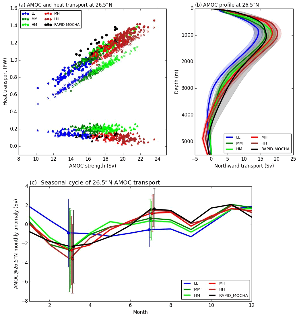
Figure 15AMOC-related metrics calculated using RapidMoc code (C. D. Roberts, 2017) consistent with the RAPID-MOCHA observations, using model years 1–100. (a) Scatter plot of each annual mean AMOC transport (x axis), with associated total heat transport (y axis) decomposed into total (circles), overturning circulation (x) and gyre transport (triangles). (b) Profile of AMOC transport with depth, shading 1 standard deviation on either side of the mean. (c) The seasonal cycle of AMOC at 26.5∘ N with annual mean value subtracted. The standard deviation is indicated for March and July only.
The depth profile of AMOC (Fig. 15b) indicates a strengthening at most depths with increased ocean resolution, with all models having a maximum at around 1000 m consistent with the observations. The shape of the AMOC profile at depth in MH/HH agrees far better with the observations (a difference of 5 Sv at 3000 m between LL and HH), which is likely to be important for global deep water masses and circulation. However, as discussed above, the peak transport at 1000 m becomes considerably stronger than observations in HH. The seasonal cycle of AMOC with annual mean removed (Fig. 15c) indicates the higher-resolution models can match the observed magnitude and phase. The AMOC minimum in March corresponds to the period of maximum variance, with reduced variability in summer.
The spatial structure of the AMOC in both depth and potential density (referenced to 2000 m) in shown in Fig. 16. The strength of the AMOC in depth space and the depth of the return flow both increase with resolution over all latitudes apart from the northern North Atlantic (50–60∘ N) where LL is marginally stronger. The depth of the southward flow deepens at higher resolutions (as seen in Fig. 15b), and at 30∘ S the AMOC is 3–5 Sv stronger at higher resolution. In density space, the AMOC is stronger everywhere at higher resolution, with clearer indication of enhanced exchange with the Nordic Seas north of 60∘ N as well as increased subpolar strength. The subtropical cell at 20–30∘ N at σ2000=34 also becomes enhanced, consistent with stronger North Atlantic Current transport. These changes are fairly typical of high-resolution model simulations (Hirschi et al., 2019), though not all models produce a stronger AMOC at higher resolution (Sein et al., 2018).
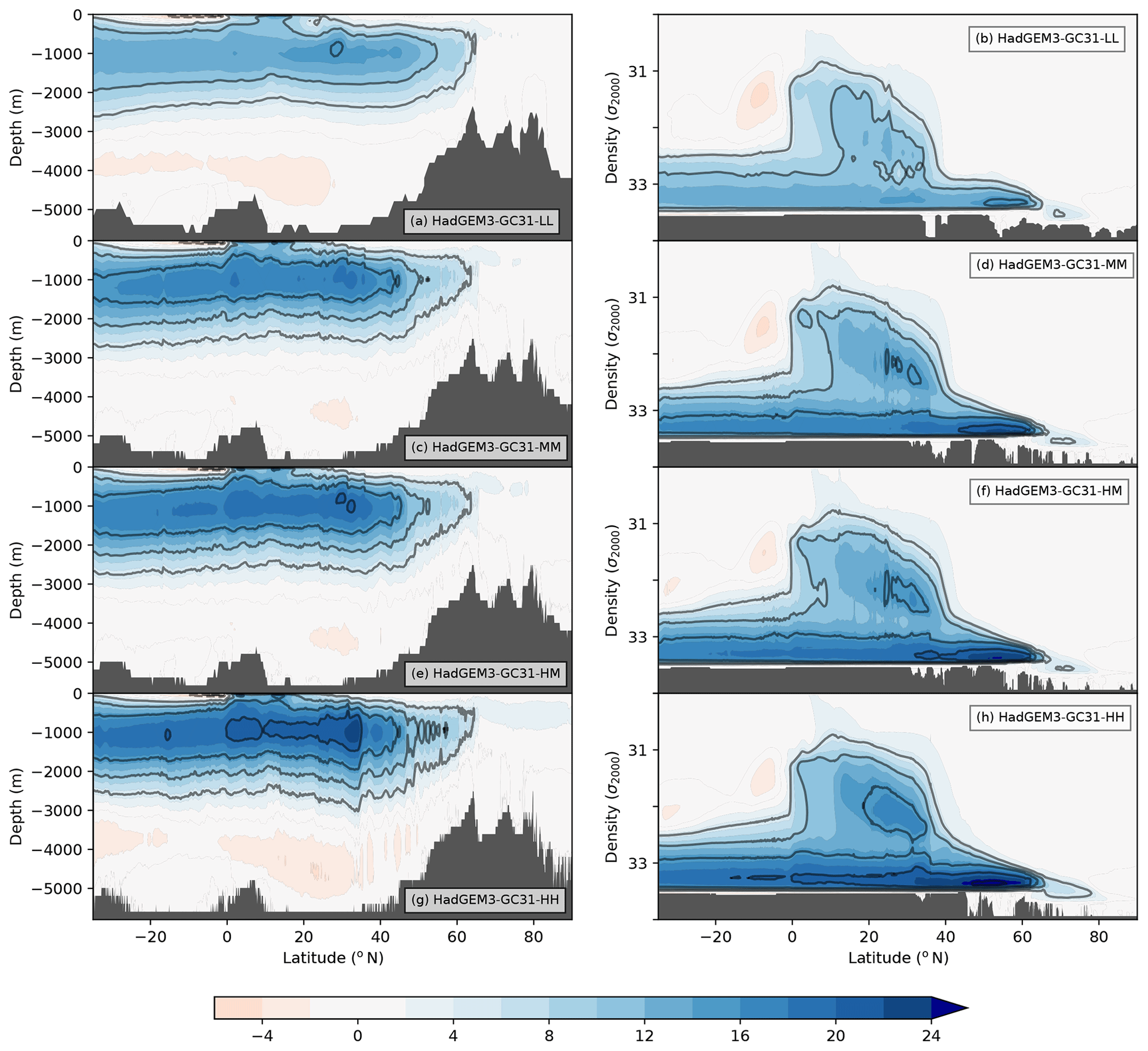
Figure 16Atlantic meridional overturning streamfunction in (left) depth coordinates and (right) potential density (σ2000) coordinates, averaged over years 50–100, in units of Sv (106 m3 s−1). The contours are at 5 Sv intervals (excluding zero).

Figure 17Ocean northward heat transport for (a) global, (b) Atlantic and (c) Indo-Pacific basins, averaged over years 50–100, separated into components: total (thick solid lines) is comprised of mean resolved advection (thick dashed lines), eddying advection (dotted lines), diffusion (Diff, thin dash-dot lines) and parameterised eddy-induced velocity (EIV, thin solid lines). The MM and HH models do not have a separately diagnosed EIV, as its parameterisation (Gent–McWilliams scheme) is switched off. For global and Indo-Pacific basins, the black circles and lines are observational estimates from Ganachaud and Wunsch (2003) with uncertainty. For the Atlantic, the black circles and lines are observational estimates from Ganachaud and Wunsch (2003) with uncertainty; the black triangle is RAPID-MOCHA (Johns et al., 2011); white diamond – Bryden and Imawaki (2001); gray circle – Talley (2003); white open circle – Lumpkin and Speer (2007); white inverted triangle – McDonagh et al. (2010); white star – Lozier et al. (2019). The coloured circles in panel (b) at 26.5∘ N correspond to the mean values using the RapidMoc calculation as in Fig. 13.
The NHT dependence on latitude is shown in Fig. 17 for the global, North Atlantic and Indo-Pacific basins, where the individual components (total, resolved advective components, diffusion and parameterised eddy-induced velocity) are also indicated. In the North Atlantic (Fig. 17b), the eddying advection component for LL is only visible near the Equator, while the eddy-induced transport associated with the Gent–McWilliams parameterisation reaches ∼0.1 PW around 40∘ N. The MM and HH models have similar eddying advective components, but the eddy-rich ocean has considerably stronger mean transport which better agrees with observations between the Equator and 40∘ N. One aspect to note is the increased HH NHT northwards of 45∘ N towards the Arctic as also seen in Roberts et al. (2016). It is unclear if this is excessive compared to observations, but if so it would imply that the ocean does not lose enough heat to the atmosphere at these latitudes.
For the global ocean (Fig. 17a), the higher resolutions have noticeably enhanced poleward transport at higher latitudes. In the Southern Ocean around 40∘ S, the balance of components is somewhat different in LL, where the resolved time-mean advection term is considerably more positive than the mean advection of the higher resolutions. In LL, this is compensated by both the parameterised eddy-induced advection (EIV) and the diffusive term (which also includes a component from the eddy parameterisation), while for higher resolutions only the eddying advection compensates, with the result that the southward transport of heat in LL is smaller. In the Indo-Pacific, the total transport has smaller differences, though at higher resolutions this is due to a stronger compensation between time-mean and eddying advective components.
3.6 Antarctic Circumpolar Current
The time evolution of the Antarctic Circumpolar Current (ACC) transport, calculated as the volume transport through Drake Passage, is shown in Fig. 18. The mean net eastward transport of 155, 90 and 125 Sv, respectively, for LL, MM and MH models compares to the recent observational range of 173±11 Sv (Donohue et al., 2016), with earlier estimates lacking a robust barotropic component (e.g. 137±8 Sv; Cunningham et al., 2003). Using the former measure, LL is closest to the observational range, while MM is only 40 % of it. Figure 18 indicates that the impact of different atmosphere resolutions is small compared to the impact of ocean resolution. A part of the deficit in the M ocean model is due to a strong countercurrent around the Antarctic shelf of about 20 Sv, together with changes to the density front, as discussed more fully in Menary et al. (2018) and Kuhlbrodt et al. (2018). The ACC in MH and HH remains lower than observed (as also seen in Small et al., 2014) – these have negligible countercurrents, but perhaps they still have too much southward heat transport (Fig. 17a) and consequently weakened density gradient, and the H ocean resolution is still only marginally eddy resolving at these latitudes (Hallberg, 2013). Despite reduced transport, however, the frontal structures associated with the ACC, some with a barotropic structure, are much more evident in the M and H ocean models (not shown).
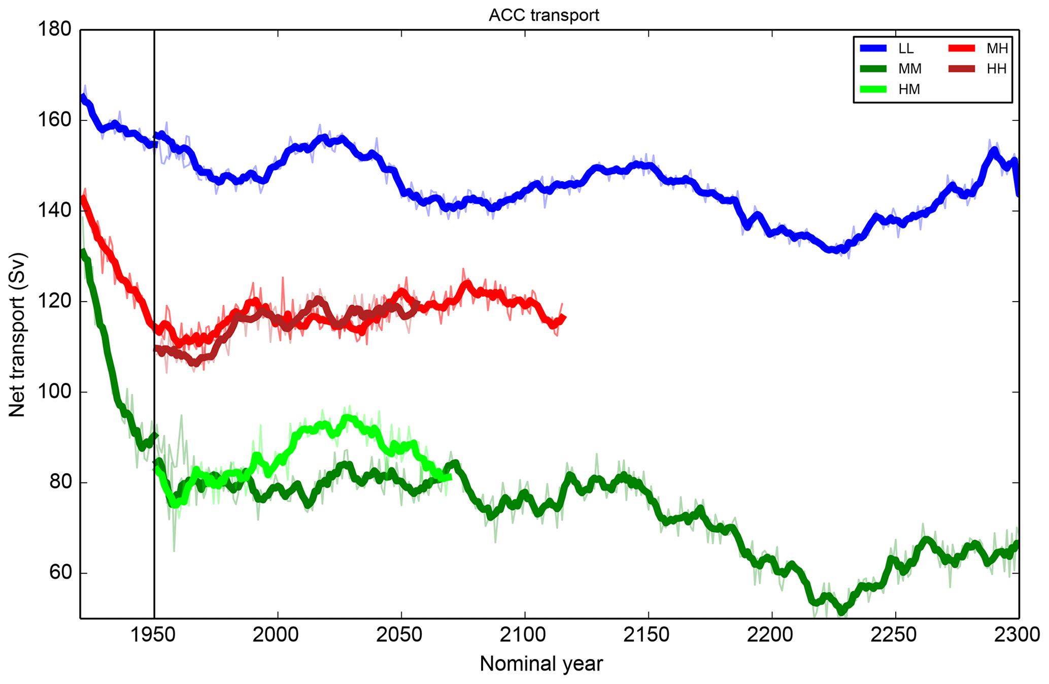
Figure 18Time series of the Antarctic Circumpolar Current (ACC) transport calculated between Antarctica and South America across Drake Passage for spinup-1950 and control-1950 simulations.
It has been shown (e.g. Kuhlbrodt et al., 2012) that the value of a constant coefficient for eddy parameterisation can influence the ACC transport via the meridional density gradient, and it is possible that the varying coefficient used in LL (Table 2) may play a similar role. Use of such a scheme in the higher-resolution models may well increase the ACC transport for similar reasons, at the expense of removing explicitly resolved mesoscale processes.
3.7 ENSO and MJO variability
As the dominant mode of interannual tropical variability, El Niño–Southern Oscillation (ENSO) is a key aspect of climate variability with worldwide impacts (Timmermann et al., 2018). Over time, there has been some improvement in modelling ENSO in global climate models (e.g. Bellenger et al., 2014), with HadGEM3-GC3.1 performance described in Williams et al. (2017), Kuhlbrodt et al. (2018) and Menary et al. (2018). Figure 19 shows the power spectrum of NINO3.4 monthly surface temperature anomalies, calculated using a periodogram method with 50 years of data in each sample and a 25-year overlap between samples, with the average power spectrum and range (shading) shown. Only the LL and MM models are shown since, as indicated in Wittenberg (2009) and Stevenson et al. (2010), 100 years is insufficient for a robust spectrum. The mean spectra from these models agree well with those from HadISST1.1 observations for 1877–2018 (Rayner et al., 2003), with the other resolutions having little obvious difference (not shown). The standard deviations of the mean NINO3.4 DJF SST from the models are all slightly higher than the observed value of 0.93.
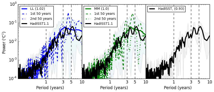
Figure 19Power spectrum of NINO3.4 surface monthly temperature variability for LL, MM resolution models and HadISST1.1 observations. The coloured line shows the mean power spectrum for all years, the dashed line shows the first 50 years, while the shading shows the range over all 50-year subsampled periods. The number in brackets is the standard deviation of the DJF mean SST in the NINO3.4 region.
The composite December–January–February (DJF) mean surface temperature patterns relating to El Niño and La Niña events are shown in Fig. 20, with events defined when the DJF NINO3.4 index exceeds ±0.7 K. There is a robust pattern to the global surface temperature anomalies which agrees well (over the ocean) with the observed HadISST1.1 dataset and over land with CRU TS (Harris et al., 2014) 2 m temperatures for 1901–2016 (Fig. 20f). The extension of the El Niño and La Niña patterns past the dateline is slightly excessive in the LL model, which is a common bias (e.g. Guilyardi, 2006; C. D. Roberts et al., 2018). The teleconnections to land surface temperature anomalies are robust over the Americas and Africa but less so over Eurasia; the models with H atmosphere tend to have stronger negative anomalies over northern Europe with El Niño, but these time series are shorter and hence have far fewer events. The surface pressure anomalies from the models (contours in Figs. 20, 21) are also consistent with the observations from HadSLP2 (Allan and Ansell, 2006).

Figure 20Composite DJF mean surface temperature (colours) for (top) El Niño and (bottom) La Niña from models and observations based on El Niño and La Niña events. The number of events sampled is shown in the title and the proportion of El Niño events classified as cold tongue (CT) and warm pool (WP). Events are defined as years when the NINO3.4 DJF SST anomaly exceeds 0.7 K. The observations are a combination of HadISST1.1 over the ocean and CRU 2 m temperatures over land, with values masked over HadISST1.1 sea ice regions. Mean sea level pressure anomalies are shown as contours with interval 0.5 hPa, with observations from HadSLP2.
The equivalent composite rainfall patterns are shown in Fig. 21 for the models and GPCP2.3 observations for 1979–2014 (Adler et al., 2018) for El Niño and La Niña events. The extension of the SST pattern into the western Pacific in LL is also evident here as excessive precipitation at the Equator in the west Pacific, with some improvement at higher resolutions. All model resolutions mirror the observed teleconnections quite faithfully, though the dry anomaly with El Niño events over South Africa is not robustly captured.
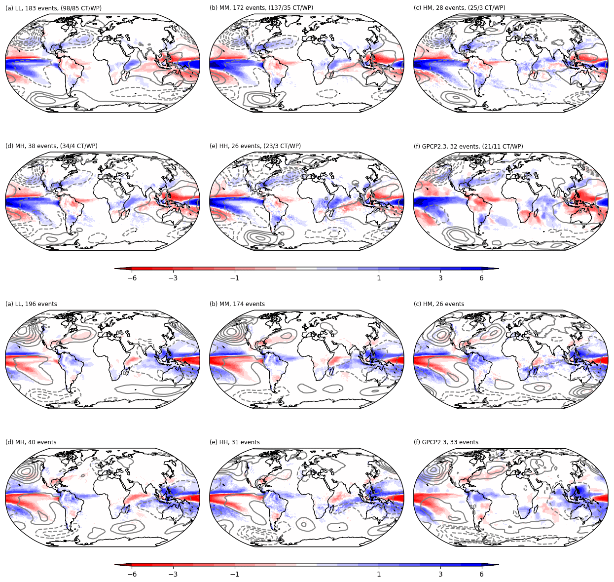
Figure 21As Fig. 18 but for DJF composites of mean precipitation (top) El Niño and (bottom) La Niña from models and GPCP2.3 precipitation, with mean sea level pressure anomalies as contours. The number of events sampled is shown in the title, along with the proportion of El Niño events classified as CT and WP. Events are defined as years when the NINO3.4 DJF SST anomaly exceeds 0.7 K.
The near-1:1 ratio of El Niño to La Niña events found in observations is replicated in the models, but the ratio of cold tongue (CT, east Pacific) to warm pool (WP, central Pacific) events, as defined by the indices in Ren and Jin (2011), is less well represented, as noted in Fig. 20 titles. The LL model has a near-1:1 ratio of such events compared to the observed 2:1, the higher-resolution ocean models have far fewer WP events compared to CT but there seems to be little systematic change with resolution.
There seems to be only minor differences in the ENSO performance in the models at different resolutions, mainly in slight differences to the SST composite. While 100 years is not long enough to assess the power spectrum, as noted previously by Wittenberg (2009) and Stevenson et al. (2010), and ENSO composites based on relatively few events can be uncertain due to internal variability (Deser et al., 2017), the composite patterns of surface temperature and precipitation show relative robustness.
The Madden–Julian Oscillation (MJO) dominates the tropical intraseasonal variability (Madden and Julian, 1971) and is characterised by eastward propagation of deep convective structures moving along the Equator with an average phase speed of around 5 m s−1 with periods between 30 and 90 d, together with other modes (Wheeler and Kiladis, 1999). The symmetric wave spectra, expressed as the ratio of raw power of outgoing longwave radiation (OLR), and a smoothed background spectra that highlights the major equatorial wave modes and their dispersion relationships compared to that of a shallow water model (represented as lines) are shown in Fig. 22a from daily NOAA observations (Lee, 2014). As shown in Menary et al. (2018) and Williams et al. (2017), the HadGEM3-GC3.1 coupled model underestimates the power in the MJO mode (wavenumbers 1–3 and periods 30–90 d) and Kelvin mode (Fig. 22b, c, d), though for the latter there is a marginal increase in power at higher resolutions. None of the resolutions are able to produce inertia–gravity (IG) waves or mixed Rossby–gravity waves in the anti-symmetric spectrum (not shown).
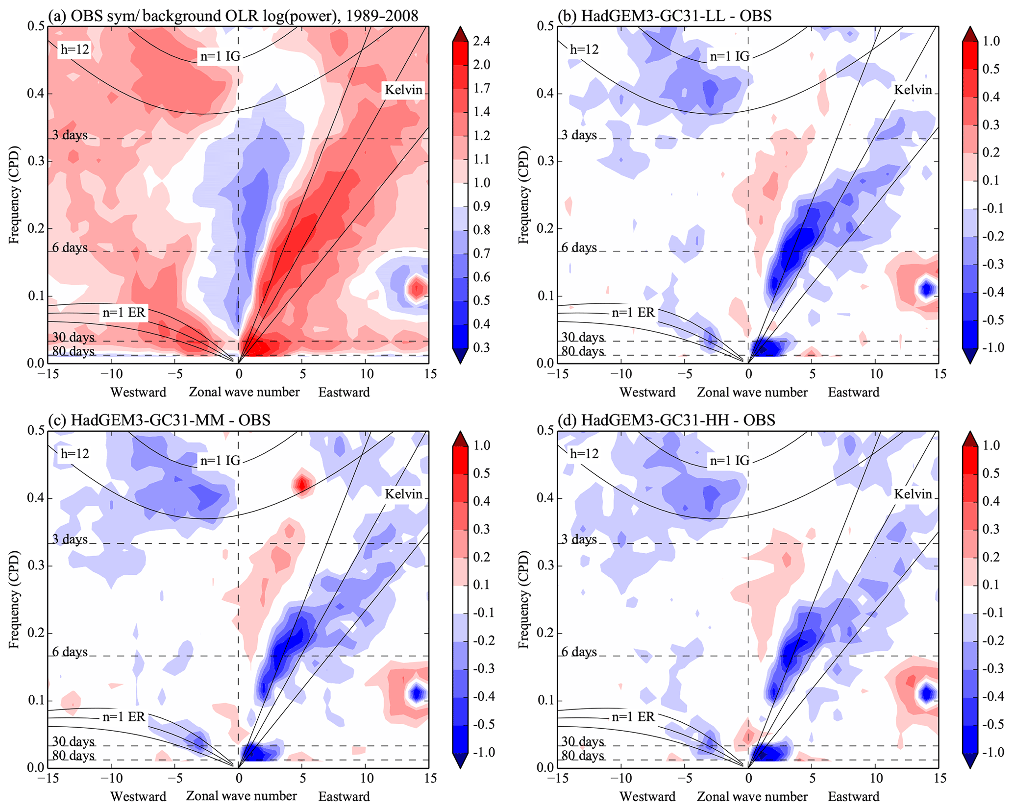
Figure 22(a) The ratio between raw power spectrum of outgoing longwave radiation (OLR) and a background spectrum from daily NOAA observations (1989–2008) averaged over 15∘ S–15∘ N. (b–d) Bias between HadGEM3-GC31-LL/MM/HH and observations, respectively, for model years 2000–2020. All values are logs of OLR power. See Wheeler and Kiladis (1999) for details. CPD indicates cycles per day.
As part of the CMIP6 HighResMIP project, a wide range of coupled model simulations with atmosphere resolutions between 250 and 50 km, and ocean resolutions from 100 to 8 km has been performed with the HadGEM3-GC3.1 model. We have shown that increased model resolution in the atmosphere and ocean can have considerable impact on climate model biases of the mean state and variability, both at the surface in terms of temperature and precipitation (Figs. 4, 7, 9, 13), as well as in the deeper ocean (Figs. 10–12).
We have demonstrated that the new CMIP6 HighResMIP experimental design, with only a multi-decadal spinup and 100-year simulation length, is sufficiently long to robustly establish some of these responses in model bias (Fig. 8). This has enabled the use an eddy-rich 8 km ocean model within the same suite of experiments to make a more comprehensive chain of resolutions and hence further test the robustness of our results. These experiments may also enable better understanding of the model adjustment process (so-called spinup from initial conditions), which tends not to be a focus of the standard CMIP simulations with a long pre-industrial spinup. This makes it harder to understand why the deep ocean adjustment process timescales may be different with different resolutions and what role these biases might play in model sensitivity to changes in forcing.
We find that increased ocean resolution is key to reducing many of the most common SST biases (Fig. 7), while a combination of ocean and atmosphere resolution significantly improves the large tropical Atlantic precipitation biases seen in typical CMIP-resolution models (Fig. 13), the latter having the potential to cause considerable uncertainty in projections of future rainfall changes.
We have also found some potential links between the biases and the evolution of the mean state. Based on previous work (Jackson et al., 2015), it seems likely that the strengthened AMOC and northward heat transport in the tropical Atlantic is linked to the improved SST biases and reduced precipitation (and ITCZ) biases, which in turn may be associated with some of the deeper ocean biases. These may also link to the different spinup behaviours seen in the different models. The initial drop in AMOC and northward heat transport in the LL model (Fig. 14) cause a cooling in the North Atlantic and Arctic, with a consequent increase in sea ice. Over time, the stronger temperature (and salinity) contrast between Equator and pole drives an increase in AMOC which gradually warms the Arctic. This increase in AMOC could be enhanced by the increased tropical Atlantic salinity bias in LL, which would increase the density of water reaching the northern North Atlantic and enable a stronger AMOC circulation to develop. Using the same initial conditions and short spinup in all experiments may enable better understanding of such adjustment processes than is generally possible in standard CMIP simulations.
While representing a substantial improvement over the length of simulation period typically used in global high-resolution experiments in the past, there are aspects of these simulations for which 100 years is not sufficient. The LL model in particular seems to take considerably longer than 30 years to quasi-equilibrate aspects of the large-scale circulation (such as AMOC), perhaps indicating that some processes are inadequately represented at this resolution. The deep ocean equilibration timescales are clearly much longer than 100 years, although there is evidence that the different resolution models trending towards different final states and the magnitude of the drifts is resolution dependent. This 100-year period is still not enough for a robust estimate of the ENSO power spectrum and variability, although the ENSO composites of surface temperature and precipitation teleconnections are apparently robust. The longer control-1950 simulations (at the lower resolutions) have been vital to test the reliability of these assertions, and hence there is probably a role for such longer simulations within the HighResMIP experimental design.
Such timescales also emphasise the importance of considering both the control-1950 and hist-1950 simulations when evaluating the models involved in HighResMIP, to properly assess model drift compared to response to forcing. An open question is whether this experimental design will enable us to identify a climate change signal in the historic and future simulations (not analysed here) by comparing these to the control simulations with constant forcing, given that the control simulations are continuing to drift. Results may be dependent on the process of interest and require new analysis methods or reference to simulations where both traditional long spinup simulations and HighResMIP experiments have been attempted.
It is unclear how robust all of the results shown here will be across a multi-model dataset. Ongoing work within Horizon 2020 PRIMAVERA project (Grist et al., 2018; C. D. Roberts et al., 2018; Vannière et al., 2018) suggests that at least for changes from 100 to 25 km ocean resolution there are robust reductions in SST and precipitation biases, while work by Griffies et al. (2015) and Small et al. (2014, 2019) does indicate some consistency in further changes to eddy-rich ocean resolutions. Further work using this multi-model ensemble within HighResMIP, in addition to comparing these simulations to their CMIP6 DECK equivalents, is ongoing and may reveal further insights into the impact of resolution and model complexity (Earth system processes such as interactive aerosols and biogeochemistry) and perhaps indicate the best trade-offs for gaining the largest model improvements for the smallest computational cost.
Most of the model data used in the following analysis are available from the CMIP6 Earth System Grid Federation and can be located using the information in M. Roberts (2018, 2017a, b, c, d) for resolutions LL, MM, HM, MH and HH, respectively. Other model resolutions are not part of the official HadGEM3-GC3.1 CMIP6 HighResMIP submission, and these data are available upon request via the CEDA-JASMIN platform.
The source code for the models used in this study, UM, JULES, NEMO and CICE, is available to use. To apply for a license for the UM, go to http://www.metoffice.gov.uk/research/approach/collaboration/unified-model/partnership (last access: November 2019), and for permission to use JULES, go to https://jules.jchmr.org (last access: November 2019). NEMO is available to download from http://www.nemo-ocean.eu (last access: November 2019), and the CICE5 model code used here is available from the Met Office code repository at https://code.metoffice.gov.uk/trac/cice/browser (last access: November 2019).
In order to implement the scientific configuration of GC3.1 and to allow the components to work together, a number of branches (code changes) are applied to the above codes. Please contact the authors for more information on these branches and how to obtain them.
Model simulations were performed by MJR, AC and RS. JS post-processed the model output into CMOR format for publication to ESGF. MJR prepared the manuscript with contributions from all co-authors.
The authors declare that they have no conflict of interest.
Malcolm J. Roberts, Jon Seddon, Pier Luigi Vidale, Reinhard Schiemann, Benoît Vannière, Alex Baker and Christopher D. Roberts acknowledge PRIMAVERA funding received from the European Commission under grant agreement 641727 of the Horizon 2020 research programme. Malcolm J. Roberts, Helene T. Hewitt, Ed W. Blockley, Pierre Mathiot and Laura C. Jackson were supported by the Met Office Hadley Centre Climate Programme funded by BEIS and Defra (GA01101). Till Kuhlbrodt was funded by the National Environmental Research Council (NERC) national capability grant for the UK Earth System Modelling project (grant no. NE/N017951/1) and by the EU Horizon 2020 Research Programme CRESCENDO project (grant agreement 641816). Pier Luigi Vidale, Reinhard Schiemann, Alex Baker and Benoît Vannière acknowledge funding from the National Environmental Research Council (NERC). Andrew Coward acknowledges funding from the ACSIS project which is supported by the Natural Environment Research Council (grant no. NE/N018044/1).
Data from the RAPID-MOCHA program are funded by the US National Science Foundation and UK Natural Environment Research Council and are freely available at http://www.rapid.ac.uk/rapidmoc (last access: May 2019) and https://mocha.rsmas.miami.edu/mocha/results/mocha-new/index.html (last access: May 2019).
We acknowledge extensive use of the supercomputers at the Met Office and the ARCHER UK National Supercomputing Service to complete the simulations and the CEDA-JASMIN platform for enabling data storage and model analysis.
We thank Paul Earnshaw, Dan Copsey, Matthew Mizielinski, Tim Graham and many other colleagues at the Met Office for help in various aspects of model simulation, data processing and analysis tools.
We would also like to thank the reviewers, Stephen Griffies, Luke Van Roekel and Justin Small, and the editor, for their time and help in improving the manuscript.
This research has been supported by the Horizon 2020 programme: PRIMAVERA (grant no. 641727) and CRESCENDO (grant no. 641816), the Joint UK BEIS/Defra Met Office Hadley Centre Climate Programme (grant no. GA01101), the National Environmental Research Council (NERC), UK Earth System Modelling (grant no. NE/N017951/1), and the Natural Environment Research Council (NERC) and ACSIS (grant no. NE/N018044/1).
This paper was edited by Richard Neale and reviewed by Stephen M. Griffies, Justin Small, and Luke Van Roekel.
Adler, R. F., Sapiano, M., Huffman, G. J., Wang, J.-J., Gu, G., Bolvin, D., Chiu, L., Schneider, U., Becker, A., Nelkin, E., Xie, P., Ferraro, R., and Shin, D.-B.: The Global Precipitation Climatology Project (GPCP) Monthly Analysis (New Version 2.3) and a Review of 2017 Global Precipitation, Atmosphere, 9, 138, https://doi.org/10.3390/atmos9040138, 2018.
Allan, R. and Ansell, T.: A New Globally Complete Monthly Historical Gridded Mean Sea Level Pressure Dataset (HadSLP2): 1850–2004. J. Climate, 19, 5816–5842, 2006.
Allan, R. P., Liu, C., Loeb, N. G., Palmer, M. D., Roberts, M., Smith, D., and Vidale, P. L.: Changes in global net radiative imbalance 1985–2012, Geophys. Res. Lett., 41, 5588–5597, https://doi.org/10.1002/2014GL060962, 2014.
Bellenger, H., Guilyardi, E., Leloup, J., Lengaigne, M., and Vialard, J.: ENSO representation in climate models: from CMIP3 to CMIP5, Clim. Dynam., 42, 1999–2018, https://doi.org/10.1007/s00382-013-1783-z, 2014.
Bischoff, T. and Schneider, T.: The Equatorial Energy Balance, ITCZ Position, and Double-ITCZ Bifurcations, J. Climate, 29, 2997–3013, https://doi.org/10.1175/JCLI-D-15-0328.1, 2016.
Bodas-Salcedo, A., Williams, K. D., Ringer, M. A., Beau, I., Cole, J. N. S., Dufresne, J. L., Koshiro, T., Stevens, B., Wang, Z., and Yokohata, T.: Origins of the Solar Radiation Biases over the Southern Ocean in CFMIP2 Models, J. Climate, 27, 41–56, https://doi.org/10.1175/jcli-d-13-00169.1, 2014.
Bodas-Salcedo, A., Hill, P. G., Furtado, K., Williams, K. D., Field, P. R., Manners, J. C., Hyder, P., and Kato, S.: Large contribution of supercooled liquid clouds to the solar radiation budget of the Southern Ocean, J. Climate, 29, 4213–4228, https://doi.org/10.1175/JCLI-D-15-0564.1, 2016.
Bryden, H. and Imawaki, S.: Ocean heat transport. Ocean Circulation and Climate, edited by: Siedler, G., Church, J., and Gould, J., Academic Press, 455–474, 2001.
Cabré, A., Marinov, I., and Gnanadesikan, A.: Global Atmospheric Teleconnections and Multidecadal Climate Oscillations Driven by Southern Ocean Convection, J. Climate, 30, 8107–8126, https://doi.org/10.1175/JCLI-D-16-0741.1, 2017.
Caldwell, P. M., Mametjanov, A., Tang, Q., Van Roekel, L. P., Golaz, J.‐C., Lin, W., Bader, D. C., Keen, N. D., Feng, Y., Jacob, R., Maltrud, M. E., Roberts, A. F., Taylor, M. A., Veneziani, M., Wang, H., Wolfe, J. D., Balaguru, K., Cameron-Smith, P., Dong, L., Klein, S. A., Leung, L. R., Li, H.-Y., Li, Q., Liu, X., Neale, R. B., Pinheiro, M., Qian, Y., Ullrich, P. A., Xie, S., Yang, Y., Zhang, Y., Zhang, K., and Zhou, T.: The DOE E3SM coupled model version 1: Description and results at high resolution. J. Adv. Model. Earth Sy., 11, https://doi.org/10.1029/2019MS001870, 2019.
Cherchi, A., Fogli, P. G., Lovato, T., Peano, D., Iovino, D., Gualdi, S., Masina, S., Scoccimarro, E., Materia, S., Bellucci, A., and Navarra, A.: Global mean climate and main patterns of variability in the CMCC-CM2 coupled model, J. Adv. Model. Earth Sy., 11, 185–209, https://doi.org/10.1029/2018MS001369, 2019.
Cunningham, S. A., Alderson, S. G., King, B. A., and Brandon, M. A.: Transport and variability of the Antarctic Circumpolar Current in Drake Passage, J. Geophys. Res., 108, 8084, https://doi.org/10.1029/2001JC001147, 2003.
Danabasoglu, G., Yeager, S. G., Bailey, D., Behrens, E., Bentsen, M., Bi, D., Biastoch, A., Böning, C., Bozec, A., Canuto, V. M., Cassou, C., Chassignet, E., Coward, A. C., Danilov, S., Diansky, N., Drange, H., Farneti, R., Fernandez, E., Fogli, P. G., Forget, G., Fujii, Y., Griffies, S. M., Gusev, A., Heimbach, P., Howard, A., Jung, T., Kelley, M., Large, W. G., Leboissetier, A., Lu, J., Madec, G., Marsland, S. J., Masina, S., Navarra, A., Nurser, A. J. G., Pirani, A., Salas y Mélia, D., Samuels, B. L., Scheinert, M., Sidorenko, D., Treguier, A.-M., Tsujino, H., Uotila, P., Valcke, S., Voldoire, A., and Wangi, Q.: North Atlantic simulations in Coordinated Ocean-ice Reference Experiments phase II (CORE-II). Part I: Mean states, Ocean Model., 73, 76–107, https://doi.org/10.1016/j.ocemod.2013.10.005, 2014.
Deser, C., Simpson, I. R., McKinnon, K. A., and Phillips, A. S.: The Northern Hemisphere Extratropical Atmospheric Circulation Response to ENSO: How Well Do We Know It and How Do We Evaluate Models Accordingly?, J. Climate, 30, 5059–5082, https://doi.org/10.1175/JCLI-D-16-0844.1, 2017.
Donohue, K. A., Tracey, K. L., Watts, D. R., Chidichimo, M. P., and Chereskin, T. K.: Mean Antarctic Circumpolar Current transport measured in Drake Passage, Geophys. Res. Lett., 43, 11760–11767, https://doi.org/10.1002/2016gl070319, 2016.
Dufour, C. O., Morrison, A. K., Griffies, S. M., Frenger, I., Zanowski, H. M., and Winton, M.: Preconditioning of the Weddell Sea polynya by the ocean mesoscale and dense water overflows, J. Climate, 30, 7719–7737, https://doi.org/10.1175/JCLI-D-16-0586.1, 2017.
Eyring, V., Bony, S., Meehl, G. A., Senior, C. A., Stevens, B., Stouffer, R. J., and Taylor, K. E.: Overview of the Coupled Model Intercomparison Project Phase 6 (CMIP6) experimental design and organization, Geosci. Model Dev., 9, 1937–1958, https://doi.org/10.5194/gmd-9-1937-2016, 2016.
Flato, G., Marotzke, J., Abiodun, B., Braconnot, P., Chou, S. C., Collins, W., Cox, P., Driouech, F., Emori, S., Eyring, V., Forest, C., Gleckler, P., Guilyardi, E., Jakob, C., Kattsov, V., Reason C., and Rummukainen, M.: Evaluation of Climate Models, in: Climate Change 2013: The Physical Science Basis. Contribution of Working Group I to the Fifth Assessment Report of the Intergovernmental Panel on Climate Change, edited by: Stocker, T. F., Qin, D., Plattner, G.-K., Tignor, M., Allen, S. K., Boschung, J., Nauels, A., Xia, Y., Bex, V., and Midgley, P. M., Cambridge University Press, Cambridge, United Kingdom and New York, NY, USA, 2013.
Fox-Kemper, B., Danabasoglu, G., Ferrari, R., Griffies, S. M., Hallberg, R. W., Holland, M., Peacock, S., and Samuels, B.: Parameterization of mixed layer eddies. III: Global implementation and impact on ocean climate simulations, Ocean Model., 39, 61–78, https://doi.org/10.1016/j.ocemod.2010.09.002, 2011.
Ganachaud, A. and Wunsch, C.: Large-Scale Ocean Heat and Freshwater Transports during the World Ocean Circulation Experiment, J. Climate, 16, 696–705, https://doi.org/10.1175/1520-0442(2003)016<0696:LSOHAF>2.0.CO;2, 2003.
Gent, P. R. and McWilliams, J. C.: Isopycnal mixing in ocean circulation models, J. Phys. Oceanogr., 20, 150–155, 1990.
Gent, P. R., Yeager, S. G., Neale, R. B. Levis, S., and Bailey, D. A.: Improvements in a half degree atmosphere/land version of the CCSM, Clim. Dynam., 34, 819, https://doi.org/10.1007/s00382-009-0614-8, 2010.
Good, S. A., Martin, M. J., and Rayner, N. A.: EN4: quality controlled ocean temperature and salinity profiles and monthly objective analyses with uncertainty estimates, J. Geophys. Res.-Oceans, 118, 6704–6716, https://doi.org/10.1002/2013JC009067, 2013.
Griffies, S. M., Pacanowski, R. C., and Hallberg, R. W.: Spurious Diapycnal Mixing Associated with Advection in a z-Coordinate Ocean Model, Mon. Weather Rev., 128, 538–564, https://doi.org/10.1175/1520-0493(2000)128<0538:SDMAWA>2.0.CO;2, 2000.
Griffies, S. M., Winton, M., Anderson, W. G., Benson, R., Delworth, T. L., Dufour, C. O., Dunne, J. P., Goddard, P., Morrison, A. K., Rosati, A., Wittenberg, A. T., Yin, J., and Zhang, R.: Impacts on ocean heat from transient mesoscale eddies in a hierarchy of climate models, J. Climate, 28, 952–977, https://doi.org/10.1175/JCLI-D-14-00353.1, 2015.
Grist, J. P., Josey, S. A., New, A. L., Roberts, M., Koenigk, T., and Iovino, D.: Increasing Atlantic Ocean Heat Transport in the Latest Generation Coupled Ocean-Atmosphere Models: The Role of Air-Sea Interaction, J. Geophys. Res.-Oceans, 123, 8624–8637, https://doi.org/10.1029/2018JC014387, 2018.
Guilyardi, E.: El Nino-mean state-seasonal cycle interactions in a multi-model ensemble, Clim. Dynam., 26, 329–348, https://doi.org/10.1007/s00382-005-0084-6, 2006.
Gutjahr, O., Putrasahan, D., Lohmann, K., Jungclaus, J. H., von Storch, J.-S., Brüggemann, N., Haak, H., and Stössel, A.: Max Planck Institute Earth System Model (MPI-ESM1.2) for the High-Resolution Model Intercomparison Project (HighResMIP), Geosci. Model Dev., 12, 3241–3281, https://doi.org/10.5194/gmd-12-3241-2019, 2019.
Haarsma, R., le Sager, P., Acosta, M., Bakhshi, R., Bretonnière, P.-A., Caron, L.-P., Castrillo, M., Corti, S., Davini, P., Exarchou, E., Garcia-Serrano, J., von Hardenberg, J., van Noyen, T., van den Oord, G., Ruprich-Robert, Y., Tourigny E., and van Weele, M.: HighResMIP versions of EC-Earth: EC-Earth3P and EC-Earth3P-HR, Description, model performance, data handling and validation, Geosci. Model Dev. Discuss., in preparation, 2019.
Haarsma, R. J., Roberts, M. J., Vidale, P. L., Senior, C. A., Bellucci, A., Bao, Q., Chang, P., Corti, S., Fučkar, N. S., Guemas, V., von Hardenberg, J., Hazeleger, W., Kodama, C., Koenigk, T., Leung, L. R., Lu, J., Luo, J.-J., Mao, J., Mizielinski, M. S., Mizuta, R., Nobre, P., Satoh, M., Scoccimarro, E., Semmler, T., Small, J., and von Storch, J.-S.: High Resolution Model Intercomparison Project (HighResMIP v1.0) for CMIP6, Geosci. Model Dev., 9, 4185–4208, https://doi.org/10.5194/gmd-9-4185-2016, 2016.
Hallberg, R.: Using a resolution function to regulate parameterizations of oceanic mesoscale eddy effects, Ocean Model., 72, 92–103, https://doi.org/10.1016/j.ocemod.2013.08.007, 2013.
Harris, I., Jones, P., Osborn, T., and Lister, D.: Updated high resolution grids of monthly climatic observations–the CRU TS3.10 Dataset, Int. J. Climatol., 34, 623–642, 2014.
Hegglin, M., Kinnison, D., Lamarque, J.-F., and Plummer, D.: CCMI ozone in support of CMIP6 – version 1.0, Version 20160711, Earth System Grid Federation, https://doi.org/10.22033/ESGF/input4MIPs.1115, 2016.
Held, I. M. and Larichev, V. D.: A scaling theory for horizontally homogenous, baroclincially unstable flow on a beta plane, J. Atmos. Sci., 53, 946–952, https://doi.org/10.1175/1520-0469(1996)053<0946:ASTFHH>2.0.CO;2, 1996.
Hewitt, H. T., Roberts, M. J., Hyder, P., Graham, T., Rae, J., Belcher, S. E., Bourdallé-Badie, R., Copsey, D., Coward, A., Guiavarch, C., Harris, C., Hill, R., Hirschi, J. J.-M., Madec, G., Mizielinski, M. S., Neininger, E., New, A. L., Rioual, J.-C., Sinha, B., Storkey, D., Shelly, A., Thorpe, L., and Wood, R. A.: The impact of resolving the Rossby radius at mid-latitudes in the ocean: results from a high-resolution version of the Met Office GC2 coupled model, Geosci. Model Dev., 9, 3655–3670, https://doi.org/10.5194/gmd-9-3655-2016, 2016.
Hirschi, J. J.-M., Barnier, B., Böning, C., Biastoch, A., Blaker, A. T., Coward, A., Danilov, S. , Drijfhout, S., Getzlaff, K., Griffies, S. M., Hasumi, H., Hewitt, H., Iovino, D., Kawasaki, T., Kiss, A. E., Koldunov, N., Marzocchi, A., Moat, B., Molines, J.-M., Myers, P. G., Penduff, T., Roberts, M., Treguier, A.-M., Sein, D. V., Sidorenko, D., Small, J., Spence, P., Thompson, L., Weijer, W., and Xu, X.: The Atlantic meridional overturning circulation in high resolution models, J. Geophys. Res., in review, 2019.
Hunke, E. C., Lipscomb, W. H., Turner, A. K., Jeffery, N., and Elliott, S.: CICE: the Los Alamos Sea Ice Model Documentation and Software User's Manual Version 5.1, LA-CC-06-012, Los Alamos National Laboratory, Los Alamos, NM, 2015.
Hyder, P., Edwards, J. M., Allan, R. P., Hewitt, H. T., Bracegirdle, T. J., Gregory, J. M., Wood, R. A., Meijers, A. J. S., Mulcahy, J., Field, P., Furtado, K., Bodas-Salcedo, A., Williams, K. D., Copsey, D., Josey, S. A., Liu, C., Roberts, C. D., Sanchez, C., Ridley, J., Thorpe, L., Hardiman, S. C., Mayer, M., Berry, D. I., and Belcher, S. E.: Critical Southern Ocean climate model biases traced to atmospheric model cloud errors, Nat. Commun., 9, 3625, https://doi.org/10.1038/s41467-018-05634-2, 2018.
Ilıcak, M., Adcroft, A. J., Griffies, S. M., and Hallberg, R. W.: Spurious dianeutral mixing and the role of momentum closure, Ocean Model., 45–46, 37–58, https://doi.org/10.1016/j.ocemod.2011.10.003, 2012.
Jackson, L. C., Kahana, R., Graham, T., Ringer M. A., Woolings, T., Mecking, J. V., and Wood, R. A.: Global and European climate impacts of a slowdown of the AMOC in a high resolution GCM, Clim. Dynam., 45, 3299, https://doi.org/10.1007/s00382-015-2540-2, 2015.
Johns, W. E., Baringer, M. O., Beal, L. M., Cunningham, S. A., Kanzow, T., Bryden, H. L., Hirschi, J. J.-M., Marotzke, J., Meinen, C. S., Shaw, B., and Curry, R.: Continuous, array-based estimates of Atlantic Ocean heat transport at 26.5 N, J. Climate, 24, 2429–2449, 2011.
Juckes, M., Taylor, K. E., Durack, P., Lawrence, B., Mizielinski, M., Pamment, A., Peterschmitt, J.-Y., Rixen, M., and Sénésis, S.: The CMIP6 Data Request (version 01.00.31), Geosci. Model Dev. Discuss., https://doi.org/10.5194/gmd-2019-219, in review, 2019.
Kato, S., Loeb, N. G., Rose, F. G., Doelling, D. R., Rutan, D. A., Caldwell, T. E., Yu, L., and Weller, R. A.: Surface irradiances consistent with CERES-derived top-of-atmosphere shortwave and longwave irradiances, J. Climate, 26, 2719–2740, 2013.
Kinter, J. L., Cash, B., Achuthavarier, D., Adams, J., Altshuler, E., Dirmeyer, P., Doty, B., Huang, B., Jin, E. K., Marx, L., Manganello, J., Stan, C., Wakefield, T., Palmer, T., Hamrud, M., Jung, T., Miller, M., Towers, P., Wedi, N., Satoh, M., Tomita, H., Kodama, C., Nasuno, T., Oouchi, K., Yamada, Y., Taniguchi, H., Andrews, P., Baer, T., Ezell, M., Halloy, C., John, D., Loftis, B., Mohr, R., and Wong, K.: Revolutionizing Climate Modeling with Project Athena: A Multi-Institutional, International Collaboration, B. Am. Meteor. Soc., 94, 231–245, https://doi.org/10.1175/BAMS-D-11-00043.1, 2013.
Klaver, R., Haarsma, R., Vidale, P. L., and Hazeleger, W.: Effective resolution in high resolution global atmospheric models for climate studies, Atmos. Sci. Lett., in review, 2019.
Kuhlbrodt, T., Smith, R. S., Wang, Z., and Gregory, J. M.: The influence of eddy parameterizations on the transport of the Antarctic Circumpolar Current in coupled climate models, Ocean Model., 52-53, 1–8, https://doi.org/10.1016/j.ocemod.2012.04.006, 2012.
Kuhlbrodt, T., Jones, C. G., Sellar, A., Storkey, D., Blockley, E., Stringer, M., Hill, R., Graham, T., Ridley, J., Blaker, A., Calvert, D., Copsey, D., Ellis, R., Hewitt, H., Hyder, P., Ineson, S., Mulcahy, J., Siahaan, A., and Walton, J.: The low-resolution version of HadGEM3 GC3.1: Development and evaluation for global climate, J. Adv. Model. Earth Sy., 10, 2865–2888, https://doi.org/10.1029/2018MS001370, 2018.
Kurtz, N. T. and Markus, T.: Satellite observations of Antarctic sea ice thickness and volume, J. Geophys. Res.-Oceans, 117, C08025, https://doi.org/10.1029/2012JC008141, 2012.
Lee, H.-T.: Climate Algorithm Theoretical Basis Document (C-ATBD): Outgoing Longwave Radiation (OLR) – Daily, NOAA's Climate Data Record (CDR) Program, CDRP-ATBD-0526, 46 pp., available at: http://www1.ncdc.noaa.gov/pub/data/sds/cdr/CDRs/Outgoing Longwave Radiation - Daily/AlgorithmDescription.pdf (last access: May 2019), 2014.
Lin, J.-L.: The double-ITCZ problem in IPCC AR4 coupled GCMs: Ocean–atmosphere feedback analysis. J. Climate, 20, 4497–4525, https://doi.org/10.1175/JCLI4272.1, 2007.
Lozier, M., Li, F., Bacon, S., Bahr, F., Bower, A., Cunningham, S., De Jong, M., De Steur, L., DeYoung, B., Fischer, J., Gary, S., Greenan, B., Holliday, N., Houk, A., Houpert, L., Inall, M., Johns, W., Johnson, H., Johnson, C., Karstensen, J., Koman, G., Le Bras, I., Lin, X., Mackay, N., Marshall, D., Mercier, H., Oltmanns, M., Pickart, R., Ramsey, A., Rayner, D., Straneo, F., Thierry, V., Torres, D., Williams, R., Wilson, C., Yang, J., Yashayaev, I., and Zhao, J.: A sea change in our view of overturning in the subpolar North Atlantic, Science, 363, 516–521, https://doi.org/10.1126/science.aau6592, 2019.
Lumpkin, R. and Speer, K.: Global Ocean Meridional Overturning, J. Phys. Oceanogr., 37, 2550–2562, 2007.
Madden, R. A. and Julian, P. R.: Detection of a 40–50 day oscillation in the zonal wind in the tropical Pacific, J. Atmos. Sci., 28, 702–708, 1971.
Madec, G., Bourdallé-Badie, R., Bouttier, P.-A., Bricaud, C., Bruciaferri, D., Calvert, D., Jérôme Chanut, J. Emanuela Clementi. E., Andrew Coward, A., Delrosso, D., Ethé, C., Flavoni, S., Graham, T., Harle, J., Iovino, D., Lea, D., Lévy, C., Lovato, T., Martin, N., Masson, S., Mocavero, S., Paul, J., Rousset, C., Storkey, D., Storto, A., and Vancoppenolle, M.: NEMO ocean engine (Version v3.6), Notes Du Pôle De Modélisation De L'institut Pierre-simon Laplace (IPSL), Zenodo, https://doi.org/10.5281/zenodo.1472492, 2017.
Mathiot, P., Hewitt, H. T., Storkey, D., Blaker, A., Roberts, M., Hyder, P., Graham, T., and Andrejczuk, M.: Sensitivity of North Atlantic circulation to bathymetry resolution, Sci. Rep., in preparation, 2019.
Matthes, K., Funke, B., Kruschke, T., and Wahl, S.: input4MIPs.SOLARIS-HEPPA.solar.CMIP.SOLARIS-HEPPA-3-2. Version 20170103.Earth System Grid Federation, https://doi.org/10.22033/ESGF/input4MIPs.1122, 2017.
McDonagh, E. L., McLeod, P., King, B. A., Bryden., H., and Valdes, S. T.: Circulation, heat, and freshwater transport at 36∘ N in the Atlantic, J. Phys. Oceanogr., 40, 2661–2678, 2010.
Meehl, G. A., Boer, G. J., Covey, C., Latif, M., and Stouffer, R. J.: The Coupled Model Intercomparison Project (CMIP), B. Am. Meteorol. Soc., 81, 313–318, https://doi.org/10.1175/1520-0477(2000)081<0313:TCMIPC>2.3.CO;2, 2000.
Meehl, G. A., Covey, C., Delworth, T. L., Latif, M., McAveney, B., Mitchell, J. F. B., Stouffer, R. J., and Taylor, K. E.: The WCRP CMIP3 multimodel dataset: A new era in climate change research, B. Am. Meteorol. Soc., 88, 1383–1394, https://doi.org/10.1175/BAMS-88-9-1383, 2007.
Megann, A.: Estimating the numerical diapycnal mixing in an eddy-permitting ocean model, Ocean Model., 121, 19–33, https://doi.org/10.1016/j.ocemod.2017.11.001, 2018.
Meinshausen, M. and Vogel, E.: input4MIPs.UoM.GHGConcentrations.CMIP.UoM-CMIP-1-2-0, Version 20160830, Earth System Grid Federation, https://doi.org/10.22033/ESGF/input4MIPs.1118, 2016.
Menary, M. B., Kuhlbrodt, T., Ridley, J., Andrews, M. B., Dimdore-Miles, O. B., Deshayes, J., Eade, R., Gray, L., Ineson, S., Mignot, J., Roberts, C. D., Robson, J., Wood, R. A., and Xavier, P.: Pre-industrial control simulations with HadGEM3-GC3.1 for CMIP6, J. Adv. Model. Earth Sy., 10, 3049–3075, https://doi.org/10.1029/2018MS001495, 2018.
Moreton, S., Ferreira, D., Roberts, M., and Hewitt, H.: Evaluating surface eddy properties in coupled climate simulations with “eddy-present” and “eddy-rich” ocean resolution, Ocean Model., in review, 2019.
Msadek, R., Johns, W. E., Yeager, S. G., Danabasoglu, G., Delworth, T. L., and Rosati, A.: The Atlantic Meridional Heat Transport at 26.5∘ N and Its Relationship with the MOC in the RAPID Array and the GFDL and NCAR Coupled Models, J. Climate, 26, 4335–4356, 2013.
Mulcahy, J. P., Jones, C., Sellar, A., Johnson, B., Boutle, I. A., Jones, A., Andrews, T, Rumbold, S., Mollard, J., Bellouin, N., Johnson, C., Williams, K., Grosvenor, D., and McCoy, D.: Improved aerosol processes and effective radiative forcing in HadGEM3 and UKESM1, J. Adv. Model. Earth Sy., 10, 2786–2805, https://doi.org/10.1029/2018MS001464, 2018.
Poli, P., Hersbach, H., Dee, D. P., Berrisford, P., Simmons, A. J., Vitart, F., Laloyaux, P., Tan, D. G. H., Peubey, C., Thépaut, J. N., Trémolet, Y., Hólm, E., Bonavita, M., Isaksen, L., and Fisher, M.: ERA-20C: An atmospheric reanalysis of the twentieth century, J. Climate, 29, 4083–4097, 2016.
Rayner, N. A., Parker, D. E., Horton, E. B., Folland, C. K., Alexander, L. V., Rowell, D. P., Kent, E. C., and Kaplan, A.: Global analyses of sea surface temperature, sea ice, and night marine air temperature since the late nineteenth century, J. Geophys. Res., 108, 4407, https://doi.org/10.1029/2002JD002670, 2003.
Ren, H.-L. and Jin, F.-F.: Niño indices for two types of ENSO, Geophys. Res. Lett., 38, L04704, https://doi.org/10.1029/2010GL046031, 2011.
Richter, I., Xie, S.-P., Wittenberg, A. T., and Masumoto, Y.: Tropical Atlantic biases and their relation to surface wind stress and terrestrial precipitation, Clim. Dynam., 38, 985–1001, https://doi.org/10.1007/s00382-011-1038-9, 2012.
Ridley, J. K., Blockley, E. W., Keen, A. B., Rae, J. G. L., West, A. E., and Schroeder, D.: The sea ice model component of HadGEM3-GC3.1, Geosci. Model Dev., 11, 713–723, https://doi.org/10.5194/gmd-11-713-2018, 2018.
Roberts, C., Waters, J., Peterson, K., Palmer, M., McCarthy, G., Frajka-Williams, E., Haines, K., Lea, D., Martin, M., Storkey, D., Blockley, E., and Zuo, W. H.: Atmosphere drives recent interannual variability of the Atlantic meridional overturning circulation at 26.5 N, Geophys. Res. Lett., 40, 5164–5170, 2013.
Roberts, C. D.: RapidMoc v1.0.1, available at: https://github.com/cdr30/RapidMoc, last access: 11 January 2017.
Roberts, C. D., Senan, R., Molteni, F., Boussetta, S., Mayer, M., and Keeley, S. P. E.: Climate model configurations of the ECMWF Integrated Forecasting System (ECMWF-IFS cycle 43r1) for HighResMIP, Geosci. Model Dev., 11, 3681–3712, https://doi.org/10.5194/gmd-11-3681-2018, 2018.
Roberts, M.: MOHC HadGEM3-GC31-LL model output prepared for CMIP6 HighResMIP, Earth System Grid Federation, navailable at: http://cera-www.dkrz.de/WDCC/meta/CMIP6/CMIP6.HighResMIP.MOHC.HadGEM3-GC31-LL (last access: May 2019), 2018.
Roberts, M.: MOHC HadGEM3-GC31-MM model output prepared for CMIP6 HighResMIP, Version 20190501.Earth System Grid Federation, https://doi.org/10.22033/ESGF/CMIP6.1902, 2017a.
Roberts, M.: MOHC HadGEM3-GC31-HM model output prepared for CMIP6 HighResMIP, Version 20190501.Earth System Grid Federation, https://doi.org/10.22033/ESGF/CMIP6.446, 2017b.
Roberts, M.: MOHC HadGEM3-GC31-MH model output prepared for CMIP6 HighResMIP, Earth System Grid Federation, available at: http://cera-www.dkrz.de/WDCC/meta/CMIP6/CMIP6.HighResMIP.MOHC.HadGEM3-GC31-MH (last access: May 2019), 2017c.
Roberts, M.: MOHC HadGEM3-GC31-HH model output prepared for CMIP6 HighResMIP, Earth System Grid Federation, available at: http://cera-www.dkrz.de/WDCC/meta/CMIP6/CMIP6.HighResMIP.MOHC.HadGEM3-GC31-HH (last access: May 2019), 2017d.
Roberts, M. J., Hewitt, H. T., Hyder, P., Ferreira, D., Josey, S. A., Mizielinski, M., and Shelly, A.: Impact of ocean resolution on coupled air-sea fluxes and large-scale climate, Geophys. Res. Lett., 43, 10430–10438, https://doi.org/10.1002/2016GL070559, 2016.
Roberts, M. J., Vidale, P. L., Senior, C., Hewitt, H. T., Bates, C., Berthou, S., Chang, P., Christensen, H. M., Danilov, S., Demory, M.-E., Griffies, S. M., Haarsma, R., Jung, T., Martin, G., Minobe, S., Ringler, T., Satoh, M., Schiemann, R., Scoccimarro, E., Stephens G., and Wehner, M. F: The Benefits of Global High Resolution for Climate Simulation: Process Understanding and the Enabling of Stakeholder Decisions at the Regional Scale, B. Am. Meteorol. Soc., 99, 2341–2359, https://doi.org/10.1175/BAMS-D-15-00320.1, 2018.
Sanchez, C., Williams, K. D., and Collins, M.: Improved stochastic physics schemes for global weather and climate models, Q. J. Roy. Meteor. Soc., 142, 147–159, https://doi.org/10.1002/qj.2640, 2016.
Schweiger, A., Lindsay, R., Zhang, J., Steele, M., Stern, H., and Kwok, R.: Uncertainty in modeled Arctic sea ice volume, J. Geophys. Res.-Oceans, 116, C00D06, https://doi.org/10.1029/2011JC007084, 2011.
Sein, D. V., Koldunov, N. V., Danilov, S., Sidorenko, D., Wekerle, C., Cabos, W., Rackow, T., Scholz, P., Semmler, T., Wang, Q., and Jung, T.: The relative influence of atmospheric and oceanic model resolution on the circulation of the North Atlantic Ocean in a coupled climate model, J. Adv. Model. Earth Sy., 10, 2026–2041, https://doi.org/10.1029/2018MS001327, 2018.
Sidorenko, D., Goessling, H. F., Koldunov, N., Scholz, P., Danilov, S., Barbi, D., Cabos, W., Gurses, O., Harig, S., Hinrichs, C., Juricke, S., Lohmann, G., Losch, M., Mu, L., Rackow, T., Rakowsky, N., Sein, D. V., Semmler, T., Shi, X., Stepanek, C., Streffing, J., Wang, Q., Wekerle, C., Yang, H., and Jung, T.: Evaluation of FESOM2.0 coupled to ECHAM6.3: Pre-industrial and HighResMIP simulations, J. Adv. Model. Earth Sy., 11, https://doi.org/10.1029/2019MS001696, 2019.
Small, R. J., Bacmeister, J., Bailey, D. A., Baker, A., Bishop, S., Bryan, F. O., Caron, J., Dennis, J., Gent, P. R., Hsu, H.-M., Jochum, M., Lawrence, D. M., Munoz Acevedo, E., diNezio, P., Scheitlin, T., Tomas, R., Tribbia, J., Tseng, Y., and Vertenstein, M.: A new synoptic scale resolving global climate simulation using the Community Earth System Model, J. Adv. Model. Earth Sy., 6, 1065–1094, https://doi.org/10.1002/2014MS000363, 2014.
Small, R. J., Curchitser, E., Hedstrom, K., Kauffman, B., and Large, W. G.: The Benguela Upwelling System: Quantifying the Sensitivity to Resolution and Coastal Wind Representation in a Global Climate Model, J. Climate, 28, 9409–9432, https://doi.org/10.1175/JCLI-D-15-0192.1, 2015.
Small, R. J., Msadek, R., Kwon, Y.-O., Booth, J. F., and Zarzycki, C.: Atmosphere surface storm track response to resolved ocean mesoscale in two sets of global climate model experiments, Clim. Dynam., 52, 2067–2089, https://doi.org/10.1007/s00382-018-4237-9, 2019.
Smeed, D., McCarthy, G., Rayner, D., Moat, B. I., Johns, W. E., Baringer, M. O., and Meinen, C. S.: Atlantic meridional overturning circulation observed by the RAPID-MOCHA-WBTS (RAPID-Meridional Overturning Circulation and Heatflux Array-Western Boundary Time Series) array at 26N from 2004 to 2017, British Oceanographic Data Centre – Natural Environment Research Council, UK, https://doi.org/10.5285/5acfd143-1104-7b58-e053-6c86abc0d94b, 2017.
Stephens, G. L., Li, J., Wild, M., Clayson, C. A., Loeb, N., Kato, S., L'Ecuyer, T., Stackhouse, P. W., Lebsock, M., and Andrews, T.: An update on Earth's energy balance in light of the latest global observations, Nat. Geosci., 5, 691–696, 2012.
Stevens, B., Fiedler, S., Kinne, S., Peters, K., Rast, S., Müsse, J., Smith, S. J., and Mauritsen, T.: MACv2-SP: a parameterization of anthropogenic aerosol optical properties and an associated Twomey effect for use in CMIP6, Geosci. Model Dev., 10, 433–452, https://doi.org/10.5194/gmd-10-433-2017, 2017.
Stevenson, S., Fox-Kemper, B., Jochum, M., Rajagopalan, B., and Yeager, S. G.: ENSO model validation using wavelet probability analysis, J. Climate, 23, 5540–5547, https://doi.org/10.1175/2010JCLI3609.1, 2010.
Storkey, D., Blaker, A. T., Mathiot, P., Megann, A., Aksenov, Y., Blockley, E. W., Calvert, D., Graham, T., Hewitt, H. T., Hyder, P., Kuhlbrodt, T., Rae, J. G. L., and Sinha, B.: UK Global Ocean GO6 and GO7: a traceable hierarchy of model resolutions, Geosci. Model Dev., 11, 3187–3213, https://doi.org/10.5194/gmd-11-3187-2018, 2018.
Talley, L. D.: Shallow, intermediate and deep overturning components of the global heat budget, J. Phys. Oceanogr., 33, 530–560, 2003.
Taylor, K. E., Stouffer, R. J., and Meehl, G. A.: An overview of CMIP5 and the experimental design, B. Am. Meteorol. Soc., 93, 485–498, https://doi.org/10.1175/BAMS-D-11-00094.1, 2012.
Timmermann, A., An, S. I., Kug, J. S., Jin, F. F., Cai, W., Capotondi, A., Cobb, K., Lengaigne, M., McPhaden, M., Stuecker, M., Stein, K., Wittenberg, A., Yun, K., Bayr, T., Chen, H., Chikamoto, Y., Dewitte, B., Dommenget, D., Grothe, P., Guilyardi, E., Ham, Y., Hayashi, M., Ineson, S., Kang, D., Kim, S., Kim, W., Lee, J., Li, T., Luo, J., McGregor, S., Planton, Y., Power, S., Rashid, H., Ren, H., Santoso, A., Takahashi, K., Todd, A., Wang, G., Wang, G., Xie, R., Yang, W., Yeh, S., Yoon, J., Zeller, E., and Zhang, X.: El Niño Southern Oscillation complexity, Nature, 559, 535–545, https://doi.org/10.1038/s41586-018-0252-6, 2018.
Titchner, H. A. and Rayner, N. A.: The Met Office Hadley Centre sea ice and sea surface temperature data set, version 2: 1. Sea ice concentrations, J. Geophys. Res., 119, 2864–2889, https://doi.org/10.1002/2013JD020316, 2014.
Treguier, A. M., Deshayes, J., Lique, C., Dussin, R., and Molines, J. M.: Eddy contributions to the meridional transport of salt in the North Atlantic, J. Geophys. Res., 117, C05010, https://doi.org/10.1029/2012JC007927, 2012.
Valcke, S., Craig, T., and Coquart, L.: OASIS3-MCT User Guide, OASIS3-MCT 3.0, Technical Report, TR/CMGC/15/38, CER-FACS/CNRS SUC URA No. 1875, Toulouse, France, 2015.
Vannière, B., Demory, M. E., Vidale, P. L., Schiemann, R., Roberts, M. J., Roberts, C. D., Matsueda, M., Terray, L., Koenigk, T., and Senan, R.: Multi-model evaluation of the sensitivity of the global energy budget and hydrological cycle to resolution, Clim. Dynam., 52, 6817–6846, https://doi.org/10.1007/s00382-018-4547-y, 2018.
Vidale, P. L., Roberts, M. J., Baker, A., Bellouin, N., Muller, O., Schiemann, R., Thornhill, G., and Vanniere, B.: Description of the resolution hierarchy of HadGEM3-GC3.1 model as used in the HighResMIP atmosphere-only experiments, Geosci. Model Dev. Discuss., in preparation, 2019a.
Vidale, P. L., Osprey, A., Lawrence, B., Roberts, M. J., Semmler, T., Scoccimarro, E., and Valcke, S.: Computational performance of PRIMAVERA and HighResMIP GCMs, Geosci. Model Dev. Discuss., in preparation, 2019b.
Voldoire, A., Saint-Martin, D., Sénési, S., Decharme, B., Alias, A., Chevallier, M., Colin, J., Guérémy, J.-F., Michou, M., Moine, M.-P., Nabat, P., Roehrig, R., Salas y Mélia, D., Séférian, R., Valcke, S., Beau, I., Belamari, S., Berthet, S., Cassou, C., Cattiaux, J., Deshayes, J., Douville, H., Franchisteguy, L., Ethé, C., Geoffroy, O., Lévy, C., Madec, G., Meurdesoif, Y., Msadek, R., Ribes, A., Sanchez-Gomez, E., and Terray, L.: Evaluation of CMIP6 DECK Experiments with CNRM-CM6-1, J. Adv. Model. Earth Sy., 11, 2177–2213, https://doi.org/10.1029/2019MS001683, 2019.
von Storch, J.-S., Haak, H., Hertwig, E., and Fast, I.: Vertical heat and salt fluxes due to resolved and parameterized meso-scale eddies, Ocean Model., 108, 1–19, https://doi.org/10.1016/j.ocemod.2016.10.001, 2016.
Walters, D., Baran, A. J., Boutle, I., Brooks, M., Earnshaw, P., Edwards, J., Furtado, K., Hill, P., Lock, A., Manners, J., Morcrette, C., Mulcahy, J., Sanchez, C., Smith, C., Stratton, R., Tennant, W., Tomassini, L., Van Weverberg, K., Vosper, S., Willett, M., Browse, J., Bushell, A., Carslaw, K., Dalvi, M., Essery, R., Gedney, N., Hardiman, S., Johnson, B., Johnson, C., Jones, A., Jones, C., Mann, G., Milton, S., Rumbold, H., Sellar, A., Ujiie, M., Whitall, M., Williams, K., and Zerroukat, M.: The Met Office Unified Model Global Atmosphere 7.0/7.1 and JULES Global Land 7.0 configurations, Geosci. Model Dev., 12, 1909–1963, https://doi.org/10.5194/gmd-12-1909-2019, 2019.
Wheeler, M. and Kiladis, G. N.: Convectively coupled equatorial waves: Analysis of clouds and temperature in the wavenumber-frequency domain, J. Atmos. Sci., 56, 374–399, 1999.
Wild, M., Folini, D., Schär, C., Loeb, N., Dutton, E. G., and König-Langlo, G.: The global energy balance from a surface perspective, Clim. Dynam., 40, 3107, https://doi.org/10.1007/s00382-012-1569-8, 2013.
Williams, K., Copsey, D., Blockley, E. W., Bodas-Salcedo, A., Calvert, D., Comer, R., Davis, P., Graham, T., Hewitt, H. T., Hill, R., Hyder, P., Ineson, S., Johns, T. C., Keen, A. B., Lee, R. W., Megann, A., Milton, S. F., Rae, J. G. L., Roberts, M. J., Scaife, A. A., Schiemann, R., Storkey, D., Thorpe, L., Watterson, I. G., Walters, D. N., West, A., Wood, R. A., Woollings, T., and Xavier, P. K.: The Met Office Global Coupled model 3.0 and 3.1 (GC3.0 & GC3.1) configurations, J. Adv. Model. Earth Sy., 10, 357–380, https://doi.org/10.1002/2017MS001115, 2017.
Wittenberg, A. T.: Are historical records sufficient to constrain ENSO simulations?, Geophys. Res. Lett., 36, L12702, https://doi.org/10.1029/2009GL038710, 2009.
Zhang, J. L. and Rothrock, D. A.: Modeling global sea ice with a thickness and enthalpy distribution model in generalized curvilinear coordinates, Mon. Weather Rev., 131, 845–861, 2003.