the Creative Commons Attribution 4.0 License.
the Creative Commons Attribution 4.0 License.
 | 05 Dec 2019
A regional atmosphere–ocean climate system model (CCLMv5.0clm7-NEMOv3.3-NEMOv3.6) over Europe including three marginal seas: on its stability and performance
Cristina Primo
Fanni D. Kelemen
Hendrik Feldmann
Naveed Akhtar
Bodo Ahrens
The frequency of extreme events has changed, having a direct impact on human lives. Regional climate models help us to predict these regional climate changes. This work presents an atmosphere–ocean coupled regional climate system model (RCSM; with the atmospheric component COSMO-CLM and the ocean component NEMO) over the European domain, including three marginal seas: the Mediterranean, North, and Baltic Sea. To test the model, we evaluate a simulation of more than 100 years (1900–2009) with a spatial grid resolution of about 25 km. The simulation was nested into a coupled global simulation with the model MPI-ESM in a low-resolution configuration, whose ocean temperature and salinity were nudged to the ocean–ice component of the MPI-ESM forced with the NOAA 20th Century Reanalysis (20CR). The evaluation shows the robustness of the RCSM and discusses the added value by the coupled marginal seas over an atmosphere-only simulation. The coupled system is stable for the complete 20th century and provides a better representation of extreme temperatures compared to the atmosphere-only model. The produced long-term dataset will help us to better understand the processes leading to meteorological and climate extremes.


Regional climate directly affects human lives and socio-economic conditions. The natural variability of the climate system impacts local weather. Due to the recent changes in the frequency and intensity of local extreme events (Tebaldi et al., 2006; Hartmann et al., 2013; Casanueva et al., 2014), like storms or heavy rainfall, we aim at a better understanding of climate system dynamics. The main components of the Earth climate system are the atmosphere, land, ocean, and rivers. To have a better representation of the interactions between the atmosphere and the rest of components of the Earth climate system, it would be necessary to couple models representing all components. However, this is highly complex since it requires combining different numerical models, which may not only bring instabilities, but also implies high computational costs. Therefore, current coupled climate systems focus only on a reduced number of these components. Since the oceans are the main boundary of the atmosphere (they cover 71 % of the Earth's surface) with a critical role in regulating energy flows (they have an enormous heat storage and transport capacity), coupled ocean–atmosphere models have been developed to better understand the interactions between the ocean and atmosphere. For example, the World Climate Research Programme (WCRP) Working Group on Coupled Modelling (WGCM) established the Coupled Model Intercomparison Project (CMIP) as a standardized experimental protocol for studying the output of coupled atmosphere–ocean general circulation models (AOGCMs) (https://pcmdi.llnl.gov/CMIP6/, last access: 2 December 2019). However, the coarse resolution of these models does not resolve important physical processes that take place at local and regional scales and that are relevant to understand extreme events like warming and precipitation trend changes. For example, marginal seas are not well represented in general circulation models (Somot et al., 2008; Li et al., 2006). In addition, it has also been demonstrated that the simulated sea surface temperature (SST) has a large spread when comparing an ensemble of AOGCMs (Dommenget, 2012) and that GCM simulations tend to underestimate high precipitation intensities (Sun et al., 2006). On the other hand, there are very high-resolution process-oriented models, like those used to forecast fog or winter storms (e.g. the Weather Research and Forecasting (WRF) model, the High-Resolution Limited Area Model (HIRLAM), or the High-Resolution Window Forecast System – HIRESW), that resolve specific smaller-scale physical processes, but the computational cost is unaffordable to run a long simulation or they miss interactive coupling with some climate system compartments (especially the marginal seas). Therefore, regional climate system models (RCSMs) present as an appropriate tool to improve the spatial scale compared to global models but keep an affordable computational cost compared to high-resolution process-oriented models.
Within the European region, different atmosphere–ocean–ice coupled RCSMs have been already run for shorter periods (a few decades). For example, Schrum et al. (2003) coupled the regional model REMO (Jacob and Podzun, 1997) and the ocean model HAMSOM (Schrum, 1997) to analyse the North and Baltic Sea, showing improvements compared to running the uncoupled HAMSOM version. Pham et al. (2014) coupled the regional model COSMO-CLM (Rockel et al., 2008) to the ocean model NEMO (Madec, 2011) for the Baltic and North Sea to evaluate the impact of these seas on the climate of Europe. They showed that the presented 2 m air temperature high biases, when compared to observations, were of the same magnitude as other COSMO-CLM studies and smaller than for the uncoupled version. Sevault et al. (2014) described and evaluated a fully coupled regional climate system model (CNRM-RCSM4) dedicated to studying Mediterranean climate variability over the period 1980 to 2012, showing a good agreement between the model and observations (e.g. seasonal cycle and the interannual variability of SST, sea level, water budget, etc.). In a recent study, Obermann et al. (2018) coupled CCLM with the NEMO set-up for the Mediterranean (NEMO-MED12) over the Med-CORDEX domain with ERA-Interim as the driving data. They showed that the coupled system was mostly able to simulate Mistral and Tramontane events with smaller biases than ERA-Interim. Akhtar et al. (2017) used that system to show the impact of the horizontal grid resolution and the dynamic ocean coupling of NEMO-MED in climate simulations with COSMO-CLM during the period from 1979 to 2009. However, all these studies focus only on a few decades, and extreme events have long return periods, so long-term simulations are more appropriate to better represent and analyse them. So far, no long-term simulation of more than 100 years with a regional climate coupled system is available. Hence, one of the goals of this work is to fill this gap.
Our aim is to improve our understanding of regional climate change in Europe and what is the added value of coupling three marginal seas (the Mediterranean, North, and Baltic Sea). Therefore, this work presents an atmosphere–ocean RCSM over Europe with an atmospheric horizontal grid resolution of about 25 km and tests its stability and performance with a simulation of more than 100 years. The added value of the coupling is analysed by comparing our simulation with a centennial atmosphere-only model run. A description of the extra costs due to the coupling compared to an atmosphere-only system is also included. We have a particular interest in better understanding changes in extreme events, like heat–cold waves and extreme precipitation; therefore, special focus is placed on analysing the performance of the system representing extremes compared to the atmosphere-only model.
The paper is structured as follows: Sect. 2 presents the regional climate system models used in this work, namely an atmosphere-only model and an atmosphere–ocean coupled model. Section 3 presents the methods and reference data used to show the stability and performance of the coupled model. Section 4 evaluates the models, distinguishing the impact of the coupling over the ocean and the European continent. Special attention is given to describing the evolution of climate change indices during the last century. Finally, Sect. 5 includes a summary with the main conclusions of the study.
This work presents an atmosphere–ocean coupled RCSM and compares it with an atmosphere-only version. This section describes the details of the different components of the RCSM: the atmospheric model, the ocean model, their set-up (lateral and boundary conditions), and how the coupling in the atmosphere–ocean system was done.
2.1 Atmospheric model
The three-dimensional non-hydrostatic limited-area atmospheric prediction model (COSMO) of the German Weather Service has a climate version, COSMO-CLM (CCLM; Rockel et al., 2008). This land–atmosphere regional climate model is based on primitive equations and accounts for a variety of physical processes with parametrization schemes (see Doms et al., 2011). In our experiment, we used the Tegen et al. (1997) aerosol climatology, the Ritter and Geleyn (1992) radiation scheme, a turbulent kinetic energy (TKE) scheme for vertical turbulence (Raschendorfer, 2001), a reduced one-moment cloud scheme following Seifert and Beheng (2001), and a convection parameterization following Tiedtke (1989). COSMO-CLM includes the soil and vegetation model TERRA, which provides soil temperature and water content (Schrodin and Heise, 2002). The atmospheric model version used in this study is CCLM v5.0 clm7 with a numerical time step of 150 s and with a 3rd-order Runge–Kutta numerical integration scheme. A sub-grid-scale sea ice mask was implemented in the CCLM coupled configuration over the North and Baltic Sea to have a better representation of sea ice by accounting for partially sea-ice-covered grid boxes.
In this study's set-up, the atmospheric lateral and top boundary conditions were provided by a simulation with the Earth system model of the Max Plank Institute (MPI-ESM version 6.1; Stevens et al., 2013). This MPI-ESM simulation was nudged (via ocean temperature and salinity) to a simulation with MPI-ESM's ocean component MPIOM (Jungclaus et al., 2013), which was forced by NOAA's atmospheric 20th Century Reanalysis (20CRv2; Compo et al., 2011) as described in Müller et al. (2015). Müller et al. (2015) ran three members, and we considered the first one (as20ncep08_r1i1p1-LR). This indirect nesting of CCLM into the 20th Century Reanalysis was necessary because of the need for consistent lateral boundary data to force the marginal seas in the RCSM.
This work compares the atmosphere-only CCLM model with an atmosphere–ocean RCSM. In the coupled version, the prescribed SST of the CCLM over the regional oceans and the fraction of sea ice in the Baltic and North Sea were replaced by the SST and sea ice fraction as simulated by coupled marginal ocean models presented in the following section, whereas the ocean models received information from the atmospheric model about the momentum and freshwater (evaporation minus precipitation), winds, solar energy, and non-solar heat flux. The MPI-ESM simulation drove both the atmosphere-only and the atmosphere–ocean RCSMs. Hence, the SST of the atmosphere-only system was prescribed with the nudged MPI-ESM SST. There was no tuning in the coupled version, and thus the configuration of the atmospheric model was the same in the coupled and uncoupled versions.
Within the Coordinated Regional Downscaling Experiment (CORDEX), different domains covering the land around the world were defined. Our study aimed to better understand the regional climate of central Europe; therefore, our simulations applied the so-called EURO-CORDEX domain (http://www.cordex.org/domains/cordex-region-euro-cordex/, last access: 2 December 2019; see Fig. 1 for a representation), with a horizontal grid spacing of 0.22∘ × 0.22∘ (∼25 km, 432 grid points) and 40 vertical levels.
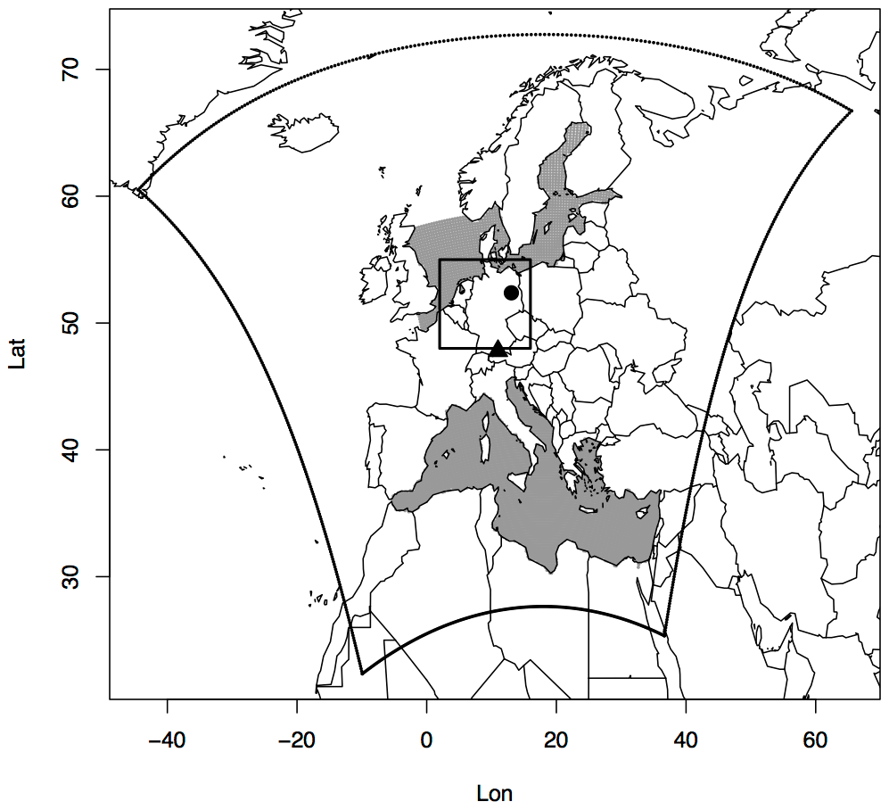
Figure 1EURO-CORDEX domain in which the coupled system runs, including the marginal seas (grey area), the mid-Europe region from the PRUDENCE project (square), and two locations of German climate stations: Potsdam (circle) and Hohenpeißenberg (triangle).
2.2 Ocean model
The Nucleus for European Modelling of the Ocean (NEMO) is a flexible tool for studying the interactions of the ocean with the atmosphere over a wide range of space scales and timescales. Within NEMO, the ocean is interfaced with a sea ice model (LIM or CICE), a passive tracer, and biogeochemical models (TOP). High-resolution configurations are available for the regional oceans in the European domain. For example, Beuvier et al. (2012) developed MED12, a regional version of the NEMO ocean engine on the Mediterranean Sea. In our simulation we used NEMO-MED12, based on NEMO version 3.6, with a resolution of 1/12∘ (∼0.083∘ ∼9 km, 688 grid points), 75 vertical levels, and a numerical time step of 720s. The initial conditions for three-dimensional potential temperature and salinity were provided by the MEDATLAS-II (Rixen, 2012) mean monthly climatology (1945–2002) in the Mediterranean Sea. The sea model was spun up in coupled mode during 20 years driven by randomly resampled MPI-ESM years in the period 1900–1910. The Black Sea and river runoff water inputs were prescribed from the climatological average of interannual data from Ludwig et al. (2009). Water exchange was in good approximation of a closed Mediterranean Ocean basin, with the Atlantic Ocean relaxed to the Levitus et al. (2005) climatology prescribed in the buffer zone.
Another NEMO set-up has been adapted to reproduce the barotropic and baroclinic dynamics, as well as the thermohaline structure, of the Baltic and North Sea basins. This is the so-called NEMO-NORDIC (Hordoir et al., 2018), whose ocean component is coupled to the sea ice model LIM3 (Vancoppenolle et al., 2009). In our study we used a NEMO-NORDIC version based on NEMO 3.3 (Dieterich et al., 2019; Gröger et al., 2019), including the LIM3 sea ice model, with a resolution of 2' (∼0.03∘ ∼ 3 km, 737 grid points), 56 vertical levels, and a numerical time step of 180 s. The initial conditions for three-dimensional potential temperature and salinity were provided by Janssen et al. (1999) and further balanced by a spin-up simulation of the period 1900–1905. The lateral boundary conditions in the North Sea were derived from the MPI-ESM simulation. Freshwater river inflow was provided from daily time series of the E-HYPE model output (Lindström et al., 2010). Neither in the NEMO-MED12 nor in the NEMO-NORDIC simulation was any drift in the surface variables detectable, including SST and sea surface salinity following balanced initialization. Figure 1 presents the domains in which the NEMO-MED and NEMO-NORDIC models run.
2.3 Coupling
In the atmosphere–ocean climate system, the atmospheric model CCLM was coupled with two configurations of NEMO: one adapted to the Mediterranean Sea (NEMO-MED12) and one to the Baltic and North Sea (NEMO-NORDIC). The coupling was done every 3 h through fully parallel communication between parallel models executed via the Model Coupling Toolkit library (MCT; Jacob et al., 2005) with the OASIS3 Model Coupling Toolkit (OASIS3-MCT; Craig et al., 2017), since this library has already been successfully used to couple the CCLM model with NEMO (Will et al., 2017). This is an interface included in CCLM based on the Message Passing Interface (MPI). It has been proved that including this library significantly improves the performance over the previous version OASIS3 because the bottleneck due to the sequential separate coupler is entirely removed (Gasper et al., 2014). During the coupling, the data on the ocean coupling grids were interpolated to the CCLM grid. At runtime, all CCLM ocean grid points located inside the interpolated area were filled with values interpolated from the ocean model, and all CCLM ocean grid points located outside the interpolated area were filled with the same external forcing data as the uncoupled system. The coupled set-up consisted of CCLM sending information to NEMO about the solar energy, non-solar heat, momentum, and freshwater fluxes, whereas it received SST from NEMO. In addition, CCLM sent the sea level pressure to NEMO-NORDIC and received the sea ice fraction. A more detailed description of the coupling strategy and its implementation can be found in Will et al. (2017) and Akhtar et al. (2019).
In addition, OASIS3-MCT offers a performance analysis tool, the LUCIA tool (Maisonnave and Caubel, 2014), that measures how much time each system component spends doing its own calculations (including send and receive operations, as well as time needed for the interpolation of fields) and how much time it waits for information coming from the other components. This tool allows for an optimization of computing resources and of the scaling of each model in the coupled system. We used the LUCIA tool to find an optimal distribution of the available number of cores used for the computation, having in mind that the model with the highest number of grid points in our system is NEMO-NORDIC (8.6 times more grid points than CCLM). Figure 2 shows an example of a configuration using 11 nodes with 36 CPUs for Mistral, the high-performance computing system for Earth system research (HLRE3) at the German High-Performance Computing Centre for Climate and Earth System Research, Germany. We assigned three nodes to CCLM, seven to NEMO-NORDIC, and one to NEMO-MED. Therefore, we assigned 3.6 times more compute resources to the coupled system than to the non-coupled system. Like this, only NEMO-MED had to wait for the exchange of the other models, while the other two models required similar times for the calculations. Figure 2 refers to the time used for send–receive operations and interpolation. To have a broader picture of the costs due to the coupling, we calculated how long it took to run just 1 d (saving the same list of CCLM variables) considering two different alternatives: (a) assuming that the number of compute resources was fixed and (b) assuming that more compute resources could be used for the coupling. In the first case, both coupled and uncoupled simulations ran in 11 nodes (CCLM ran in three nodes in the coupled system). Like this, the coupled simulation ran in around 5 min, whereas the uncoupled ran in around 1 min. In the second case, CCLM ran in three nodes for both coupled and uncoupled simulations. In this case, it took around 2 min to run the uncoupled system. Therefore, for this example, the coupled system was around 5 times slower given the same number of available nodes but around 2.5 times slower when more resources were used.
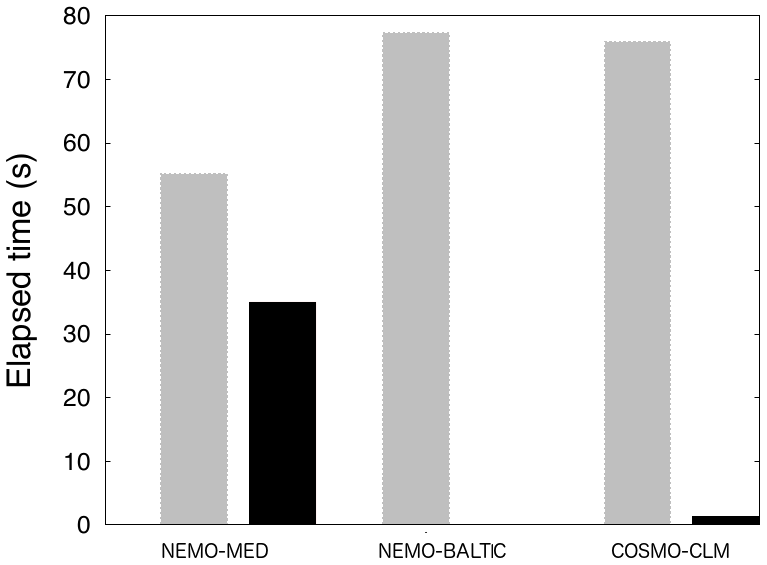
Figure 2Computing time used for the exchange of each of the OASIS coupled model components. Grey bars show calculation time and black bars show waiting time.
For the centennial simulation, we used 576 CPUs optimally distributed as follows: 24×13 CPUs were assigned to CCLM, 12×8 to NEMO-MED12, and 14×12 to NEMO-NORDIC. With this configuration, each simulated month required around 1.5 h in total, which implied 78 d to run the complete centennial simulation (110 years). To obtain the optimized computational performance of a coupled system, Will et al. (2017) show that the coupling method plays a larger role compared to the computing architecture or the individual model components.
Our aim was to test whether the coupled system is stable over the whole century and whether the coupled simulation, including the hydrosphere component represented by the Mediterranean, North, and Baltic Sea, improves not only the global MPI-ESM-LM simulations, but also performs at least as well as the atmosphere-only model.
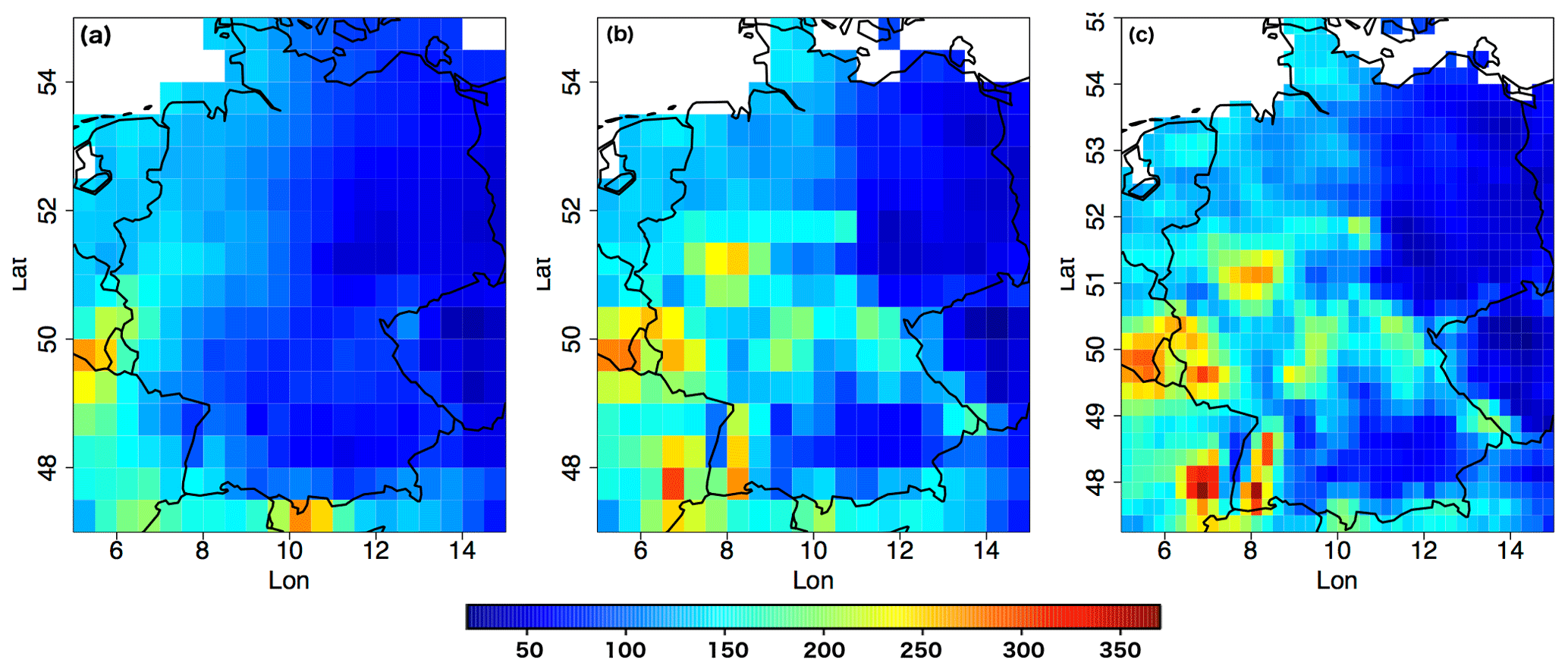
Figure 3Gridded total precipitation observations for January 1995: (a) CRU data (0.5∘ × 0.5∘), (b) E-OBS data upscaled to 0.5∘ × 0.5∘, and (c) E-OBS data with original resolution (0.25∘ × 0.25∘).
3.1 Methods
The stability of the coupled atmosphere–ocean RCSM was tested with a spatio-temporal analysis of a centennial simulation (1900–2009). The analysis consisted of a study of the temporal series evolution, annual cycles, spatio-temporal density distributions, and spatial patterns of three variables of interest: sea surface temperature, 2 m air temperature, and total precipitation. Results were compared to the same analysis obtained with an atmosphere-only (CCLM) version simulation over the same period, run within the national research project on climate prediction MiKlip (Mittelfristige Klimaprognosen; Marotzke et al., 2016). The temporal series analysis helped us to detect any bias or drift of the atmosphere–ocean simulation compared to the atmosphere-only simulation, and the spatial analysis was to detect if the system behaves differently according to the area of interest.
Regarding the quality of the coupled model, we compared our simulation with different reference datasets (see the next section for more details). Rather than a point-by-point comparison with the reference data, we would like to know if the system represents the reference value distributions well. For this purpose, we compared the density distributions and box plots of our system with those obtained from observational datasets. We analysed the marginal seas separately, also distinguishing among seasons. Regarding the land, different relevant areas have been used in the literature for regional climate studies over Europe; e.g. within the European project PRUDENCE (Prediction of Regional scenarios and Uncertainties for Defining EuropeaN Climate change Risks and Effects; Christensen, 2005) eight regions were defined: British Isles, the Iberian Peninsula, France, mid-Europe, Scandinavia, the Alps, the Mediterranean, and eastern Europe. Since we aim to improve our understanding of the regional climate in Germany, we showed results in the mid-Europe PRUDENCE region.
We are also interested in high-impact phenomena: heavy precipitation, dry spells, and heat waves. The joint CCl/CLIVAR/JCOMM Expert Team (ET) on Climate Change Detection and Indices (ETCCDI) suggested a list of 27 core climate change indices based on daily temperature values and daily precipitation amounts (Karl et al., 1999; Zhang et al., 2011). The definition of these indices can be found on the web page of the project (etccdi.pacificclimate.org/list_27_indices.shtml). We computed these indices using the freely available R package RClimDex, which is developed, maintained, and provided by Xuebin Zhang and Yang Feng at the Climate Research Division of the Environment and Climate Change Canada. In addition to the computation of the indices, it also provides simple quality control for the daily input data. We also analysed how the distributions of these indices were represented compared to the distribution of the indices obtained with the observed dataset.

Figure 4Sea surface temperature annual means over the marginal seas in our 20th century coupled simulation (CCLM-NEMO) between 1900 and 2005 compared to observations (HadISST and OISSTv2), to the atmosphere-only CCLM simulation (with SSTs prescribed by the driving MPI-ESM nudged to observations), and an ensemble mean (white line) and spread (shaded area) from CMIP5 simulations. (a) Mediterranean Sea and (b) Baltic and North Sea.
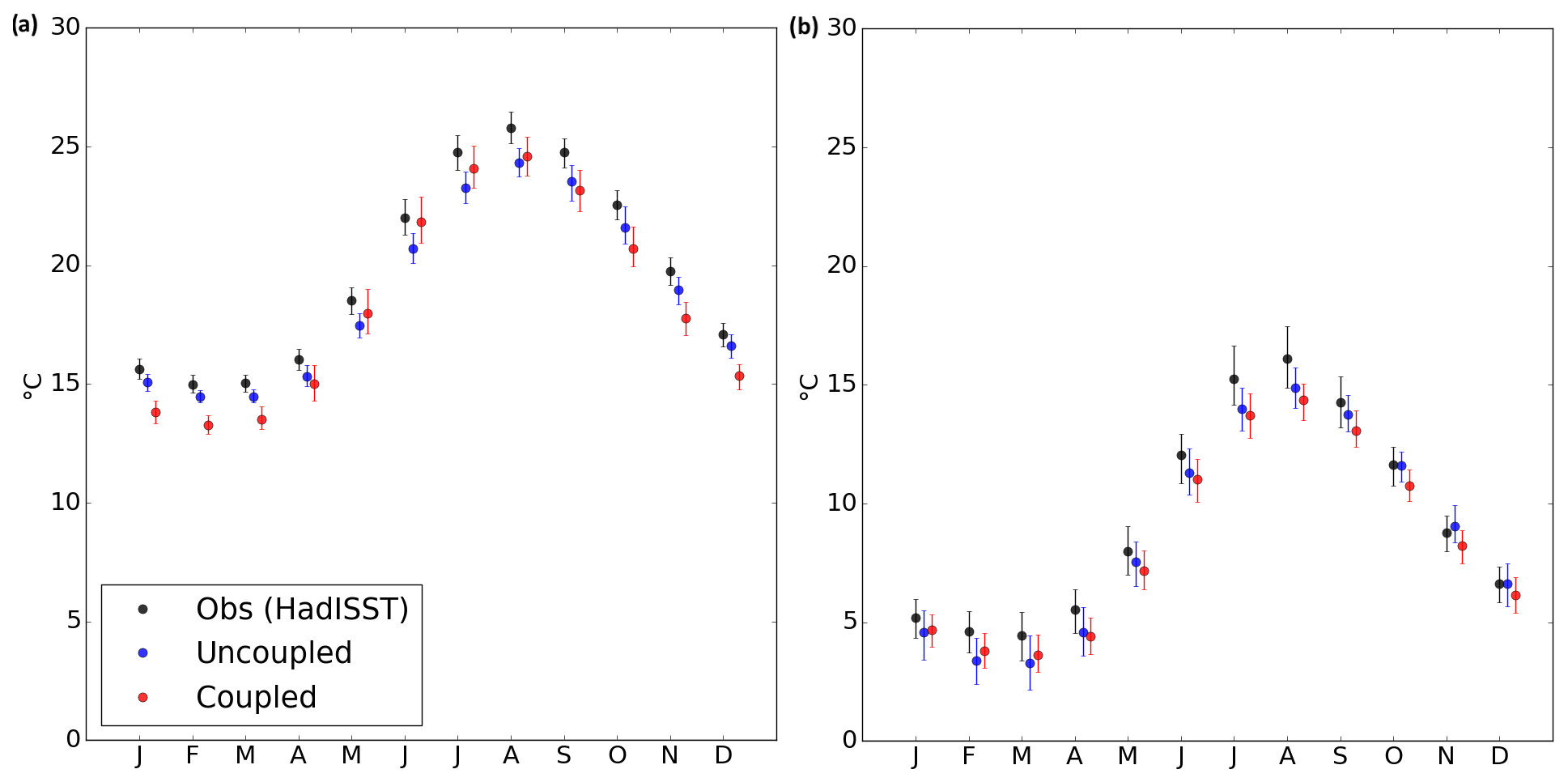
Figure 5Annual cycle during the 20th century of the spatially averaged SST values in the marginal seas: (a) Mediterranean Sea; (b) Baltic and North Sea. Dots represent the mean monthly value and intervals show the 10th and 90th percentiles.
3.2 Reference data
Two centennial reference datasets were available: the gridded Climatic Research Unit (CRU) observation time series (TS, 2017) produced at the University of East Anglia and the station observations from the Deutscher Wetterdienst Climate Data Center (DWD-CDC). The CRU dataset is available for the period January 1901 to December 2016 (Harris et al., 2014) and consists of monthly data on high-resolution (0.5∘ × 0.5∘) grids. In this work, version 4.01 data (CRU, 2017) is used. Our simulations had a higher resolution (0.22∘ × 0.22∘), and therefore a necessary upscaling prevents us from validating the high-resolution information available in the model when comparing to CRU. However, there is no available higher-resolution gridded dataset covering the complete century. If we wanted to compare model data with gridded observations with similar spatial resolution, we would have to consider shorter periods. For example, the gridded data E-OBS dataset (Haylock et al., 2008) is available at a spatial resolution of 0.22∘. However, it covers only half of our period of interest (from 1950 onwards). It is worthy to remark that in any case none of these observational datasets are perfect and that they also differ from each other. For example, Fig. 3 shows a comparison of the monthly mean in January 1995, when a flood event happened over Germany. The figure illustrates the information loss regarding the event through upscaling compared to the 0.22∘ resolution. This fact can penalize our system when comparing it with CRU, especially for the first half of the century, in which E-OBS data are not available. Nevertheless, this will not affect the coupled and atmosphere-only model intercomparison.
To compare our coupled data with centennial observations with higher quality, we considered historical daily station observations. The Climate Data Center (CDC) of the German National Weather Service (Deutscher Wetterdienst, DWD) provides free access to quality-controlled observations from DWD climate stations (DWD-CDC, 2017). We chose nine stations with less than 15 % missing values, covering the complete period (1900–2009), that were well distributed over Germany. Figure 1 shows two of these stations with no data gap that are located at two different altitudes and distances to the seas: Potsdam (circle, altitude: 81 m) and Hohenpeißenberg (triangle, altitude: 977 m). For the sake of brevity, this work presents a comparison of the RCSMs only for these two stations, but similar conclusions were reached with the other seven stations.
Over the ocean, unfortunately, there is no high-resolution observed dataset for the complete period. Hence, we used the Hadley Centre Sea Ice and Sea Surface Temperature dataset (HadISST; Rayner et al., 2003) developed by the Met Office Hadley Centre for Climate Prediction and Research with a 1∘ resolution as a reference. In addition, we compared the sea surface temperature over the Mediterranean with the NOAA Optimum Interpolation Sea Surface Temperature v2 (OISSTv2; Reynolds et al., 2002) for the available decades (1981–2009). We used these data even though they only cover a few decades because the sea surface temperature of the CCLM atmosphere-only simulation is not independent from the HadISST observations (they were used to obtained the MPI-ESM driving simulation). Besides the observations, we also compared the coupled system over the marginal seas with a multi-model ensemble consisting of the first member (r1i1p1) of eight CMIP5 models.
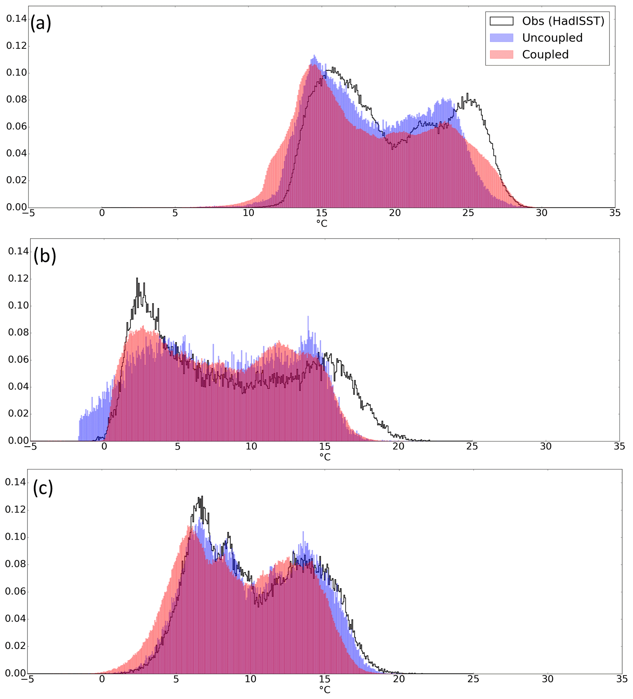
Figure 6Density histograms of SST values in the marginal seas: (a) Mediterranean Sea, (b) Baltic Sea, and (c) North Sea. Note that in the case of the Baltic Sea the grid points containing sea ice were not considered. CRU is represented in white, the coupled system in red, the uncoupled in blue, and the data overlapping in purple.
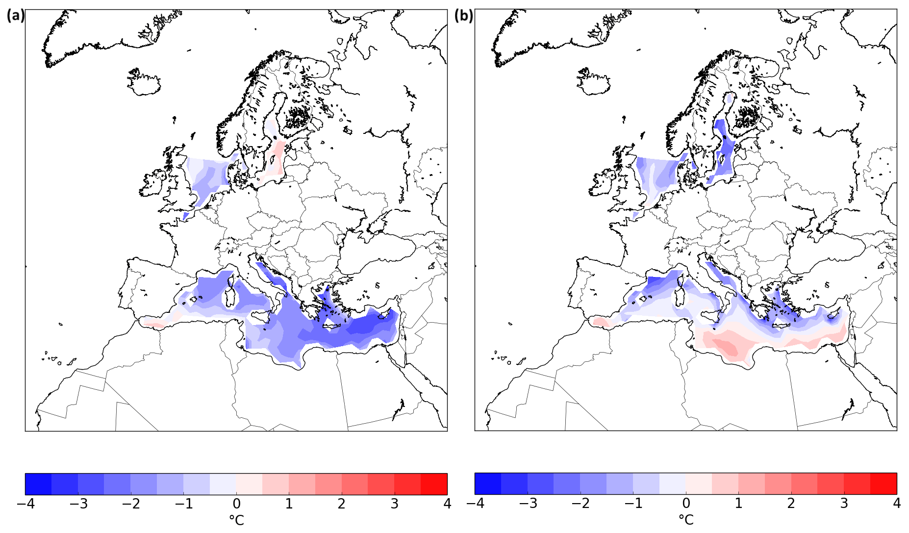
Figure 7Spatial distribution of coupled simulation–observation SST differences in (a) winter and (b) summer.
We based our analyses on three variables: sea surface temperature, 2 m air temperature, and total precipitation. The behaviour over ocean and land is presented separately. We refer to the atmosphere-only model (CCLM) as uncoupled and the atmosphere–ocean model (CCLM-NEMO) as coupled.
4.1 Sea surface temperature
We analysed the temporal evolution of the SST over the marginal seas (Mediterranean and Baltic–North Sea) to see if there is any drift or evolving bias in the coupled system over the ocean (Fig. 4). The SST of the coupled version used the simulated NEMO SST, whereas the SST of the uncoupled version was from the global system MPI-ESM. The long-term SST time series of our coupled system shows a stable system, although the annual mean SST values are colder than the observations (HadISST) and also than in the uncoupled system (from the global system) in both basins. The global system MPI-ESM-LM simulation is not independent from the HadISST observations; therefore, NOAA OISSTv2 was also included in the comparison for the available last 3 decades (1981–2009). Despite the cold bias, the regional coupled system follows the evolution of the observed SST values. In the Mediterranean, it even matches the ensemble mean of the CMIP5 global simulations, and in the Baltic, it is within the spread of this ensemble. Therefore, the SST values from the coupled system have at least as good quality as the values of an average global model, with the advantage of having higher resolution, which preferably improves the model results, especially in the land–sea transition zone. Improving the quality of the averaged global model was expected since global circulation models contain ocean models that are not well suited to shelf seas like the Baltic and North seas.
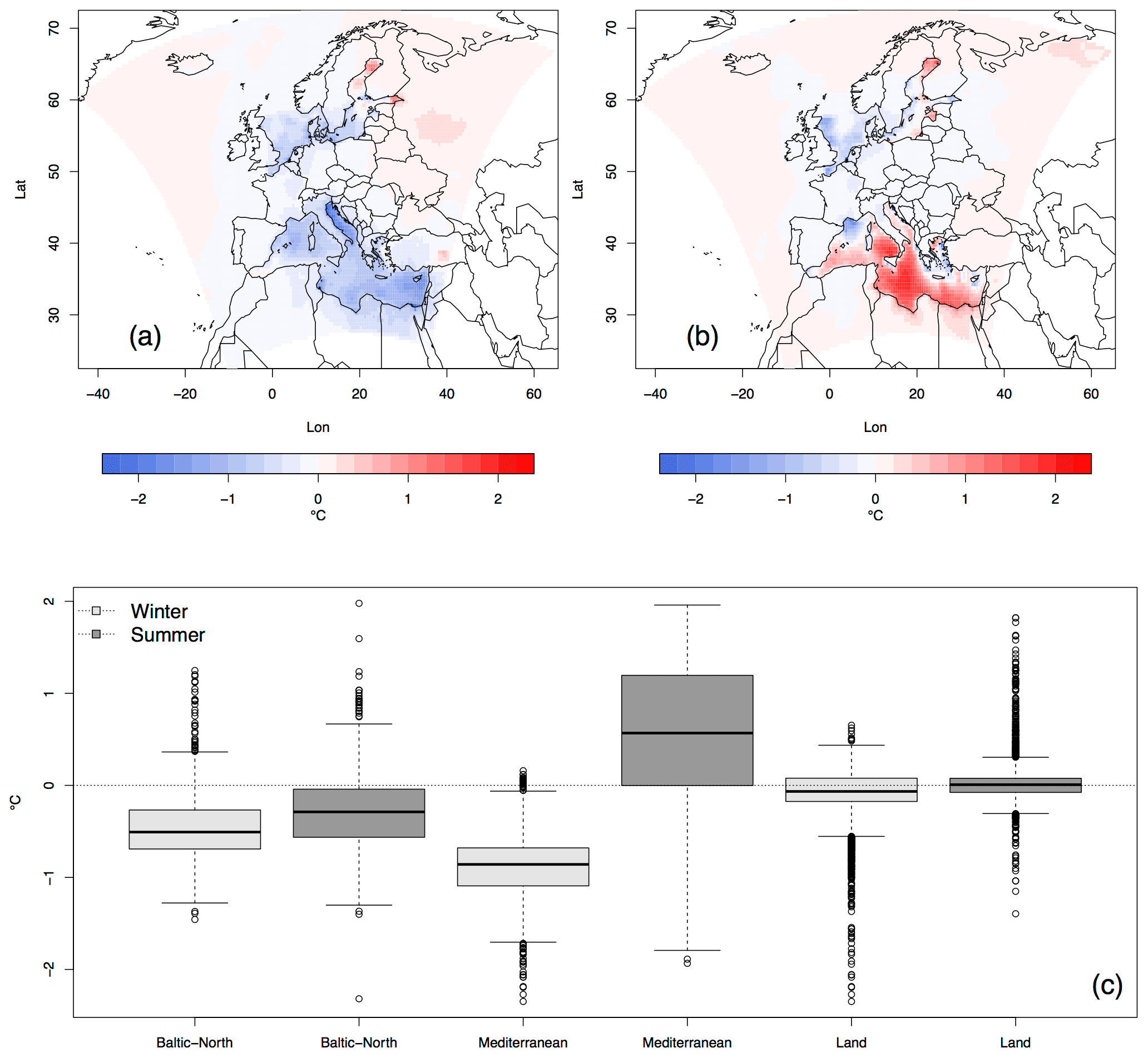
Figure 8Coupled minus uncoupled simulation 2 m air temperature monthly mean (∘C) averaged over the 20th century during winter (a) and summer (b). Box plots represent the distributions of the monthly mean over the marginal seas and land separately (c). The box ends at quartiles, the horizontal line represents the median, and the points are values more than 1.5 times the interquartile range from the end of the box.
Figure 5 shows a good representation of the SST annual cycle for both basins. In the Mediterranean, the coupled system is colder in winter and warmer in summer than observations and global simulations. In the Baltic and North Sea basin, the coupled system is colder throughout the year.
The density histograms of the three marginal seas summarize both the spatial and the temporal distribution of the SST values (Fig. 6). Since the Baltic and North seas have different climatologies in winter due to the presence of ice (the Baltic Sea is colder and less salty than the North Sea), we have analysed their histograms separately. In the Mediterranean Sea, the distribution of model data and observations has a similar shape, namely a double maximum representing summer and winter temperatures. Comparing the modelled and the observed histograms, both the coupled and uncoupled models capture the main aspects of the SST distribution. The regional coupled simulation has a wider distribution than the observations, which is made up of a well-fitting upper range and a shift towards cooler temperatures at the lower range. In comparison with the uncoupled version, the coupled system better represents the upper extremes but has a colder bias in the lower tail. The distribution shape of the uncoupled dataset is very similar to the observation shape, which was expected with the forcing SSTs constrained by the 20CR and thus the observed SSTs. Still, the uncoupled model has a cold bias in both tails.
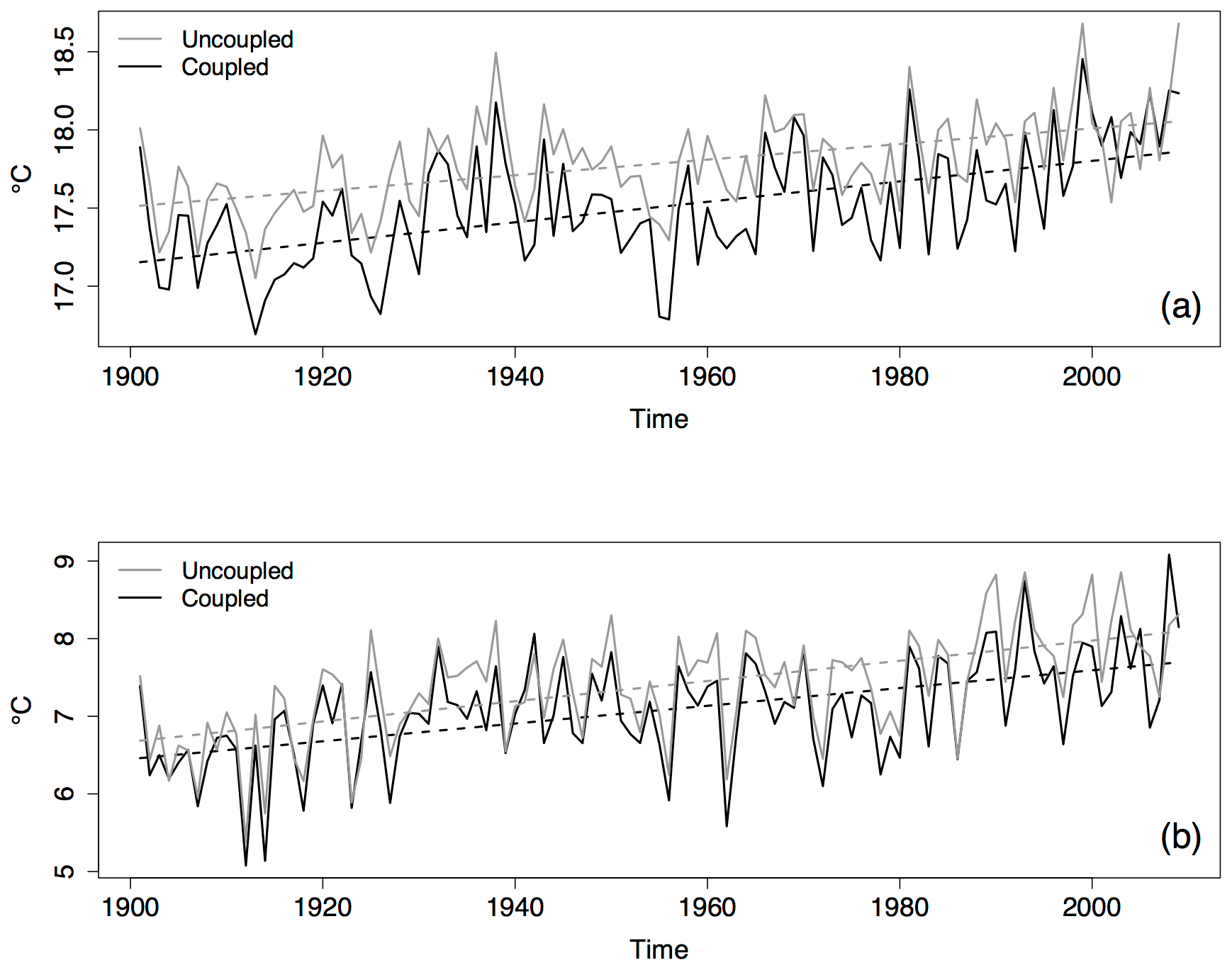
Figure 9Temporal evolution of the annual 2 m air temperature averaged over (a) the Mediterranean Sea and (b) the Baltic and North Sea. Dashed lines are linear fits.
The SST of the coupled version in the Baltic and North Sea comes from the ocean NEMO-NORDIC model, which includes sea ice and freezing–melting processes via a sea ice model. This leads to an improvement in the lower tail of the distribution over the Baltic compared to the uncoupled system that provides much colder temperatures. Both systems have a cold bias in the upper tail. Regarding the North Sea, the coupled model shows a colder bias compared to the uncoupled model.
The spatial distribution of the regional coupled system's SST bias shows that the modelled seas, as previously seen, are cooler than observations in all seasons (Fig. 7; spring and autumn are not shown). Nevertheless, during winter the basin of the Baltic Sea has a warm bias, and during summer the Mediterranean Sea has a gradient in the bias field from south to north.
Explaining the SST bias of the coupled system compared to the uncoupled SST is not straightforward and is out of the scope of this study. Many factors may have an impact on the coupled SST (internal dynamics of NEMO, salinity changes, initialization of the ocean, deeper mixing layer depth, etc.). Nonetheless, given that the coupled system was not retuned, the results of the transient RCSM simulation are promising.
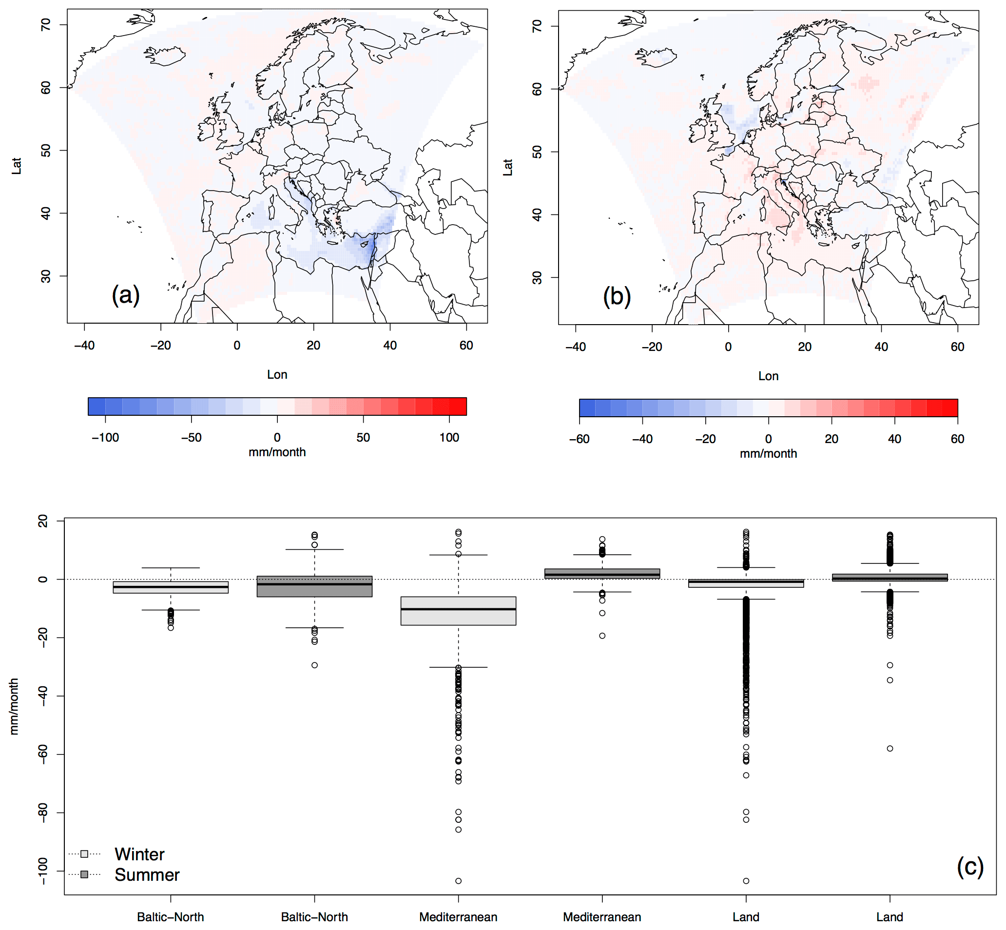
Figure 10Total precipitation coupled–uncoupled system monthly sum difference averaged over (a) winter and (b) summer for the period 1901–2009. Box plots (c) represent the distribution of these differences over the marginal seas and land separately. The box ends at quartiles, the horizontal line represents the median, and the points are values more than 1.5 times the interquartile range from the end of the box.
4.2 2 m air temperature
This section analyses how the coupled system propagates the interactive SST information into the atmosphere and over land, in particular the impact on 2 m air temperatures. Figure 8 shows the differences of the 2 m air temperature monthly mean between the coupled and uncoupled systems averaged during winter (a) and summer (b) for the period 1901–2009. The plots show differences up to almost 2.4 ∘C. The coupled system gives colder temperatures over the Mediterranean Sea during winter and warmer temperatures during summer, with the exception of the French coast and north-east coast (regions influenced by cold wind systems like Mistral and Meltemi). Regarding the Baltic and North Sea, the summer and winter difference patterns are similar. The coupled model provides colder temperatures over the North Sea and western parts of the Baltic Sea, whereas there are warmer temperatures over the north and eastern parts of the Baltic Sea. The box plots (c) represent the distribution over the marginal seas separately and over land for each season over the whole period. The plot shows that the spread of the differences on the Baltic–North Sea is similar during the year, and the coupled system is mainly colder. The highest spread of differences happens in the Mediterranean in summer, when the coupled version is warmer. In winter the spread is smaller and the coupled system is colder. Regarding the land, in summer the median is about zero and there is very small spread, showing mainly no difference between the systems. However, there are some outliers for which the coupled system shows higher temperatures (with up to 2 ∘C difference). In winter the differences are slightly more noticeable, and the main outliers are negative, showing that the coupled simulation allows for colder temperatures.
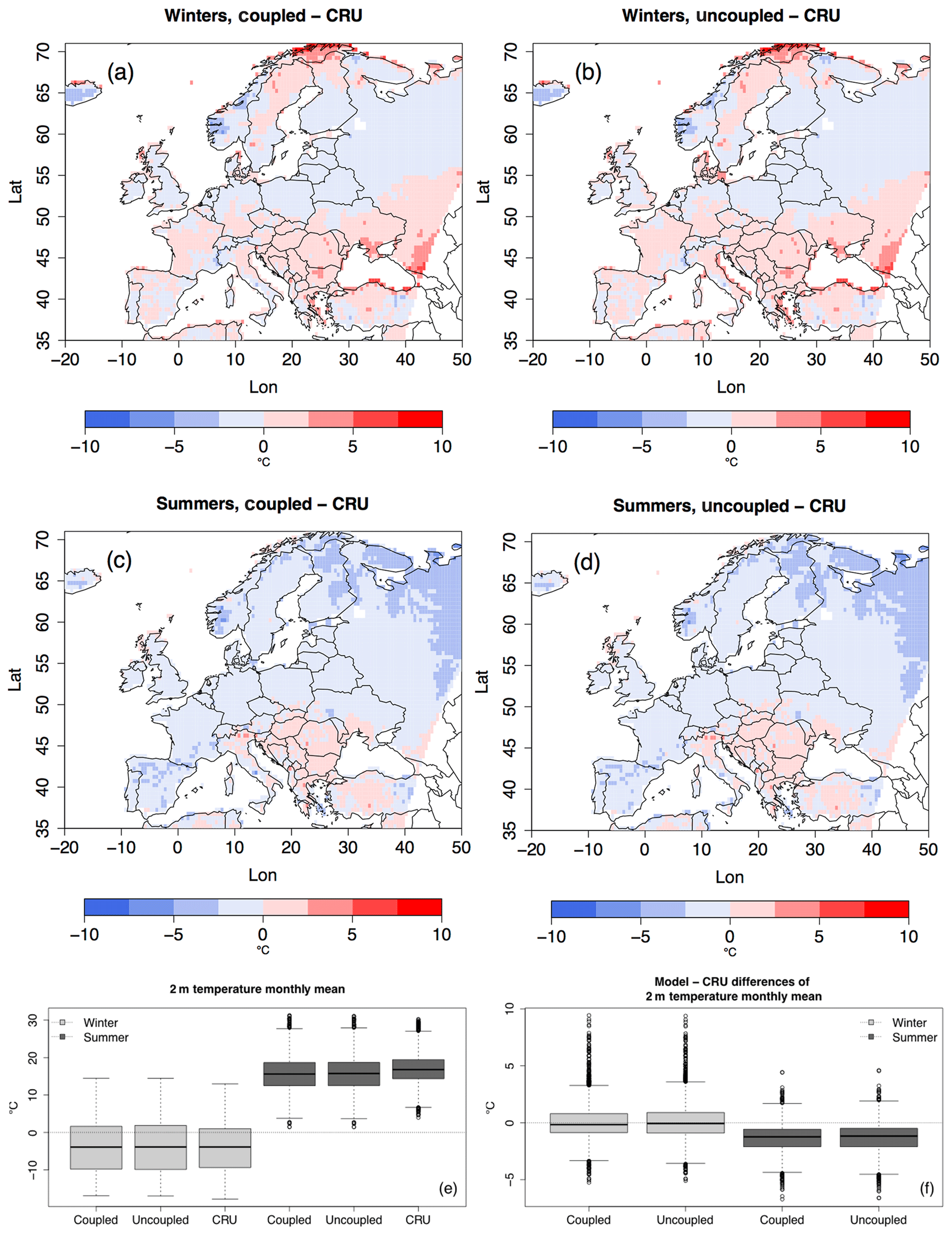
Figure 11The 2 m air temperature coupled system–CRU data differences (a, c) and the uncoupled system and CRU data (b, d) during winter (a, b) and summer (c, d) for the 20th century. Box plots of the 2 m air temperature (e) and box plots of the regional model–CRU difference (f). Box plots follow the same criterion as in previous figures.
Figure 9 shows the temporal evolution of the annual 2 m air temperature averaged over the marginal seas. The figure shows that both the coupled and uncoupled systems represent a similar positive trend and have strongly intercorrelated time series. To better understand how the 2 m air temperature of the coupled system responds to changes in the SST, Kelemen et al. (2019) ran a few sensitivity experiments using perturbed SST in the uncoupled system. They showed a positively oriented impact of SST disturbance on 2 m air temperatures.
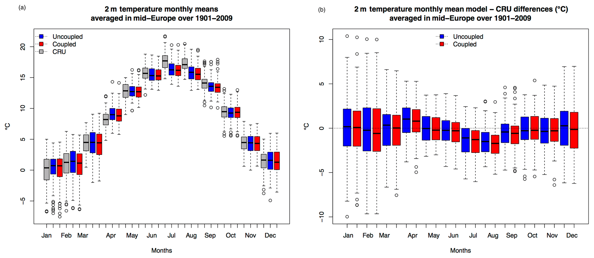
Figure 12Box plots showing the annual cycle during the 20th century of the 2 m air temperature monthly means averaged over mid-Europe for the CRU observations (grey), the uncoupled system (blue), and the coupled system (red) (a), as well as the annual cycle of the model errors compared to CRU observations over mid-Europe (b).
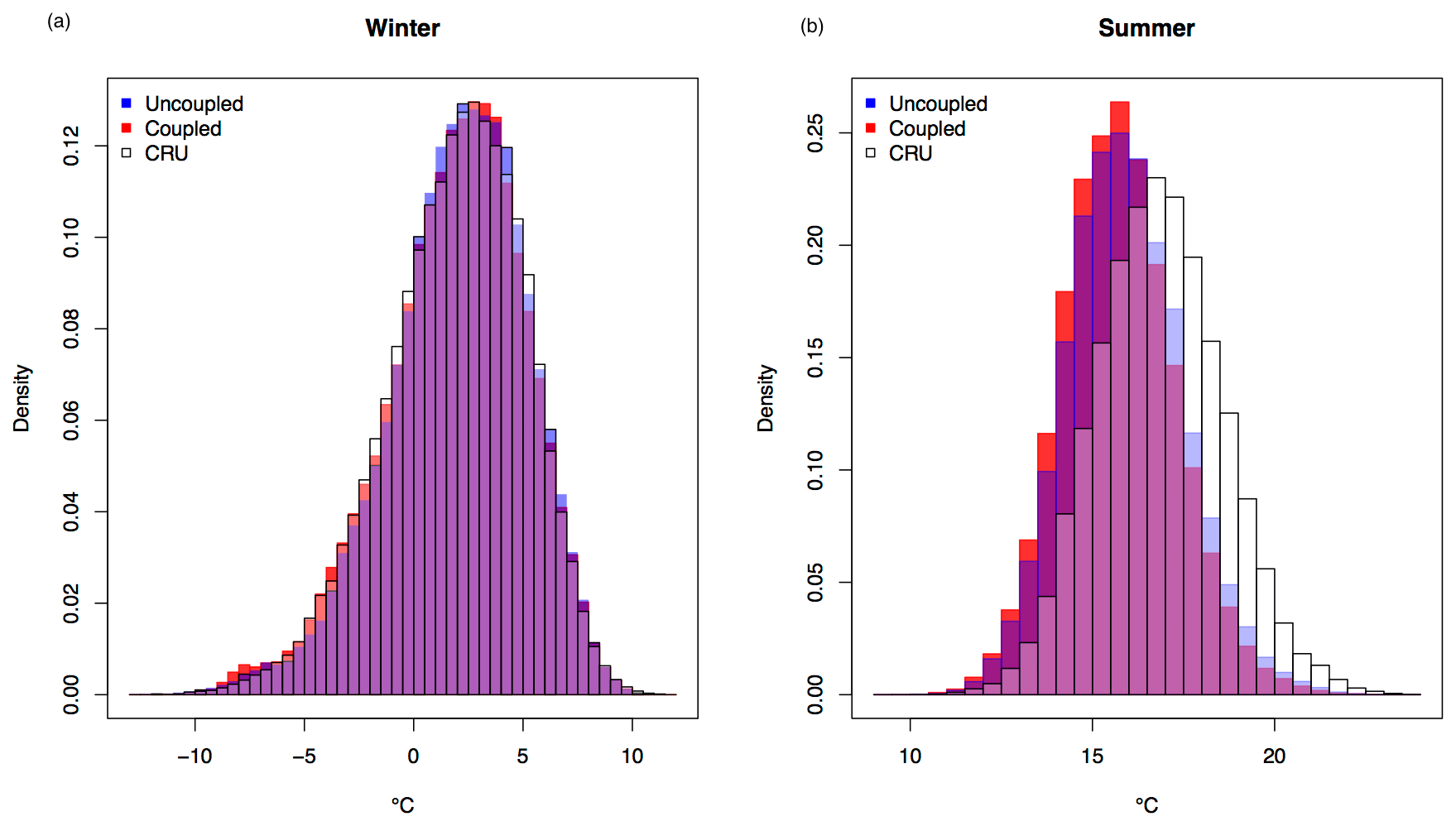
Figure 13The 2 m air temperature density histograms of the coupled and uncoupled systems compared to the CRU data over the PRUDENCE area mid-Europe during the 20th century in winter (a) and summer (b). The coupled system is represented in red, the uncoupled in blue, CRU in white, and the data overlapping in purple.
4.3 Total precipitation
Figure 10 represents the winter and summer precipitation differences between the coupled and the uncoupled system. The largest differences are in the eastern Mediterranean in the winter season, with large areas with 20 to 50 mm month−1 less precipitation in the coupled than in the uncoupled simulation. In summer, however, the coupled system gives more precipitation in most Mediterranean areas. Regarding the North Sea, the uncoupled simulation gives in general more precipitation than the coupled. The differences in the Baltic are smaller, being slightly more appreciable in summer than in winter. The precipitation differences over the seas are in concordance with the differences of 2 m air temperature. Box plots (Fig. 10c) show the monthly difference distributions over the marginal seas and land separately. The spread in the Baltic–North Sea is higher in summer with more positive outliers, whereas in the Mediterranean it is higher in winter (with generally small monthly precipitation amounts in summer) with more negative outliers (higher precipitation for the uncoupled system). The differences over land are smaller in general with large outliers in winter. The latter emerged near the Mediterranean coast, where the coupled system is drier, and in the Alpine region, where the coupled system is wetter.
To better understand how the total precipitation of the coupled system responds to changes in the SST, Kelemen et al. (2019) did sensitivity studies showing a higher response in total precipitation than in the 2 m air temperature. They also showed an added value in the seasonal precipitation sums of the coupled system during winter over the eastern part of the domain.
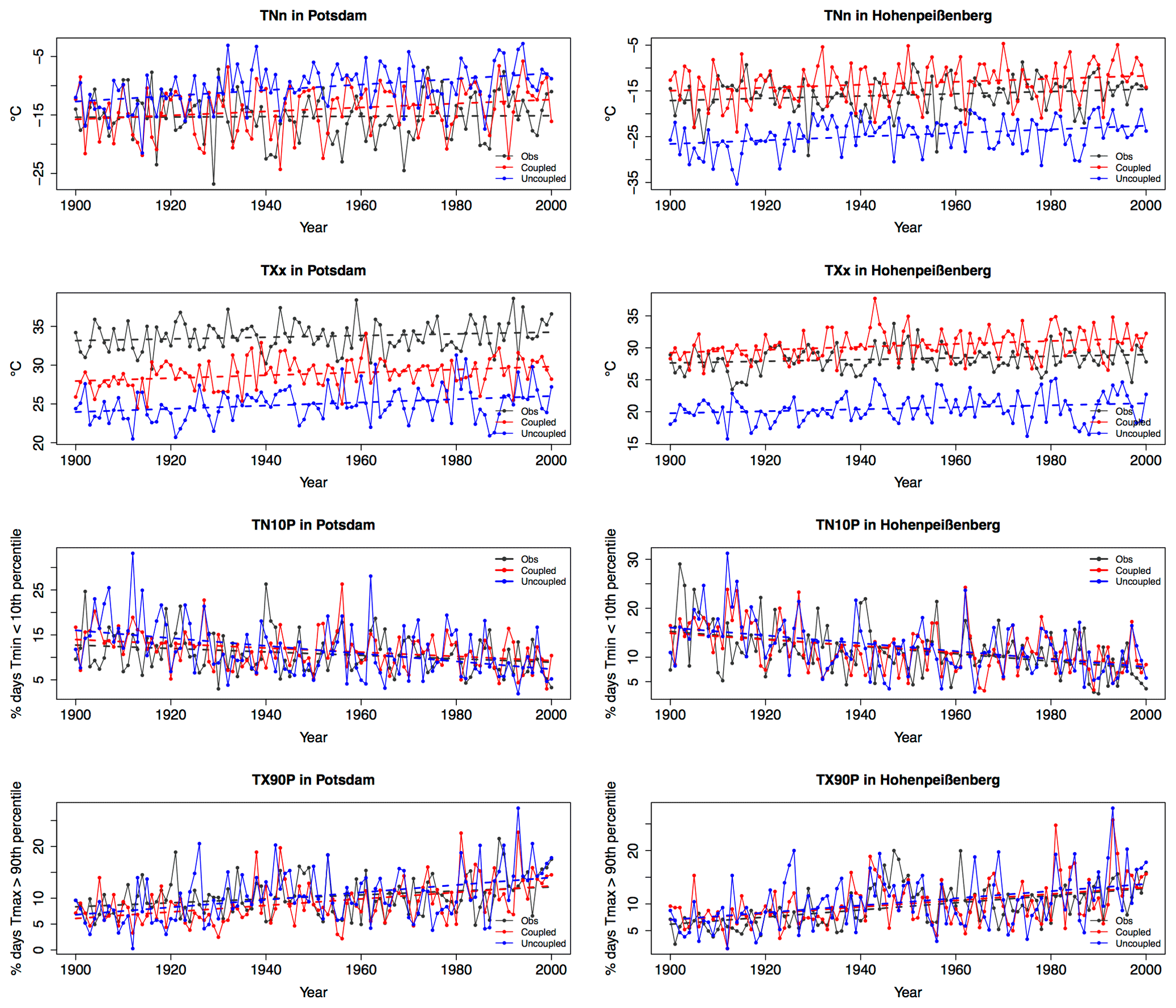
Figure 14Temporal evolution of four climate change indices at two stations in Germany, Potsdam (81 m) and Hohenpeißenberg (977 m). TNn represents the annual minimum value of daily minimum temperature; TXx represents the annual maximum value of daily maximum temperature; TX90p represents the percentage of days when the maximum temperature is above the calendar-day 90th percentile centred on a 5 d window for the base period 1961–1990; and TN10p represents the percentage of days when the minimum temperature is below the calendar-day 10th percentile centred on a 5 d window for the base period 1961–1990. Linear trends are shown as dashed lines.
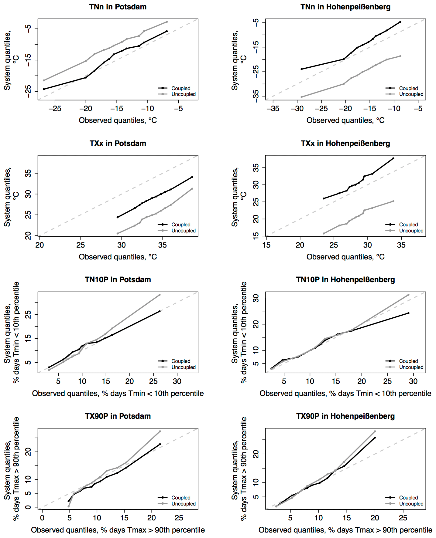
Figure 15Quantile–quantile plots of the extreme indices shown in Fig. 14. The diagonal represents the perfect case.
4.4 Model-observation comparisons
This section studies the performance of the coupled system in Europe. For this purpose, we compared the model data (coupled and uncoupled systems) with the observed CRU dataset. Data coming from coupled and uncoupled systems were interpolated to the 0.5∘ × 0.5∘ CRU grid, and only grid points defined in all three datasets were considered. Errors of the 2 m air temperature of the coupled and uncoupled systems when compared to the CRU observations for winter and summer, the 2 m air temperature distributions, and the distributions of the 2 m air temperature errors are shown in Fig. 11. In winter, there is no clear positive or negative bias (Fig. 11a–b). However, in summer the coupled and uncoupled systems are colder than the CRU observations, apart from the Alpine region and the south-east area, where both systems are warmer (Fig. 11c–d). Box plots show a good representation of the observed distribution (Fig. 11e). In winter distributions are similar and the main differences appear in summer, when the systems show slightly colder values in the low temperature range. The differences also show a similar distribution for the coupled and uncoupled systems (Fig. 11f). As mentioned in Sect. 4.2, the 2 m air temperature differences between the coupled and non-coupled systems are below 2.5 ∘C; however, box plots show that the differences compared to CRU are much higher, up to 10 ∘C in winter. In summer more than 75 % of the 2 m air temperature given by the systems is colder than the observations. In winter there is no clear bias, and box plots are centred around the zero value. Nevertheless, there are more extreme higher values (longer upper tail in winter showing higher temperatures for the systems compared to the observations).
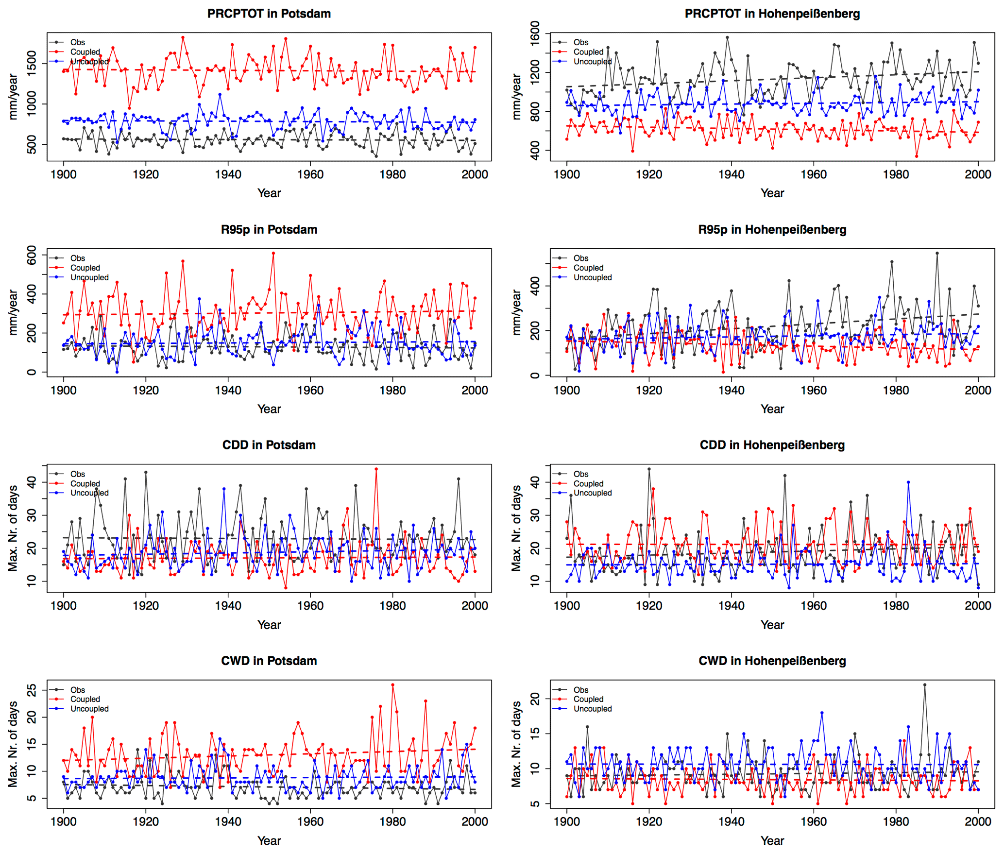
Figure 16Temporal evolution of four climate change indices related to precipitation at two German stations: Potsdam (81 m) and Hohenpeißenberg (977 m). PRCPTOT represents the annual total precipitation on wet days, R95p is the annual total PRCP when the daily precipitation (RR) is above the 95th percentile of precipitation on wet days in the 1961–1990 period, CDD is the maximum length of dry spell (maximum number of consecutive days with RR<1 mm), and CWD is the maximum length of wet spell (maximum number of consecutive days with RR≥1 mm). Linear trends are shown as dashed lines.
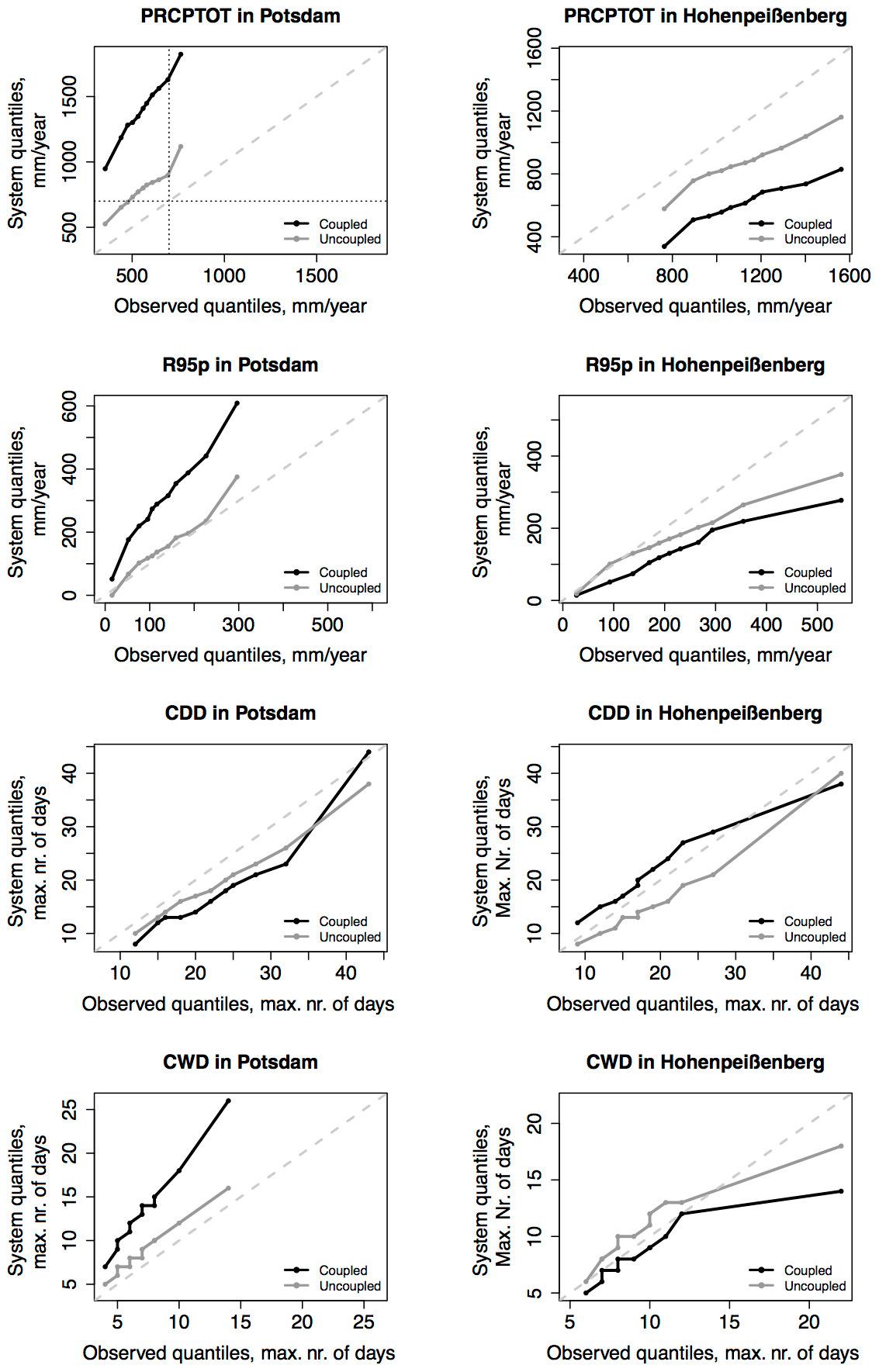
Figure 17Quantile–quantile plots of the extreme indices shown in Fig. 16. The diagonal represents the perfect case.
We are interested in the impact that the coupling may have in the 2 m air temperature performance over Europe, in particular over the PRUDENCE region mid-Europe. Figure 12 represents box plots corresponding to the annual cycle of the monthly 2 m air temperature averaged over mid-Europe for the 20th century (a) and the distributions of the differences of the model values minus the CRU observations (b). Both systems show similar distributions as the CRU data in winter but colder distributions in summer. The differences are centred around the zero value in winter and below zero in summer; that is, on average the winter is better represented by the regional systems than the summer. However, the spread is much bigger in winter than in summer; that is, in cases in which the regional systems differ from the CRU observed data, the differences are higher in winter than in summer. Compared to the complete domain (Fig. 11e), the spread of the distributions (box height) over mid-Europe is smaller than over the whole domain, since over mid-Europe the temperatures do not differ as much as they do when comparing the temperatures over the southern and northern parts of the whole domain. In addition, the extreme cases (points) are also milder compared to the whole domain since the summers are not as hot as in southern regions like the Iberian Peninsula or north Africa, and winters are not as cold as in northern regions. Figure 12 also points out winter outliers. In this case, for example, the coupled system better estimates the coldest temperatures in January over mid-Europe. This is a result that was not appreciated when comparing the whole domain. However, the box plots do not give us detailed information about the different 2 m air temperature values. To analyse in more detail the differences in the tails of the distributions, Fig. 13 shows the density histograms of the 2 m air temperature of the coupled and uncoupled systems compared to the CRU data over mid-Europe. Blue bars represent the uncoupled system, red bars the coupled system, white bars the CRU observations, and purple the intersection. As shown in the left tail of the winter distribution, the coupled system estimates the values around −5 ∘C well, although it overestimates those around −8 ∘C. Nevertheless, both systems show a good fit in winter but a colder bias in summer.
4.5 Extreme events
The effect of coupling the marginal seas has been shown to be a useful tool to simulate regional climate over Europe and study extreme events, like Vb cyclones during the period 1979–2014 (Akhtar et al., 2019). In this section we will focus on the representation of climate indices during the whole 20th century. The monthly CRU data cannot be used to analyse extreme events like heat–cold waves or dry–wet spells. Instead, observed station data provided by the German Weather Service (DWD-CDC, 2017) were considered in this study. We computed core climate change indices suggested by the ETCCDI over the 20th century for the coupled and uncoupled systems, as well as for long-term series of station data located in Germany. We chose indices having an impact on human lives; for example, Fig. 14 shows the temporal evolution of four climate change indices related to extreme temperatures: annual minimum temperature TNn, annual maximum temperature TXx, information on warm spells TX90p (defined as the percentage of days when the maximum temperature is above the calendar-day 90th percentile centred on a 5 d window for the base period 1961–1990), and finally information on cold spells TN10p (defined as the percentage of days when the minimum temperature is below the calendar-day 10th percentile centred on a 5 d window for the base period 1961–1990). To compute the 10th and 90th percentiles for each calendar day, a bootstrap procedure was used to avoid possible inhomogeneity across the in-base and out-base periods (Zhang et al., 2005). Linear trends of the indices are given too. Figure 14 shows the stable evolution of the indices in the coupled version, the capturing of the trends, and the improvement of the uncoupled version for the TNn and TXx indices, especially for the higher station. The coupled system detects the increase in temperature during the century, the increase in the percentage of days with maximum temperatures above the 90th percentile, and the percentage of days with a minimum temperature below the 10th percentile.
Figure 15 compares the distributions of these indices for the coupled and uncoupled systems against the observations based on the quantiles. The diagonal represents the perfect case, assuming that observations are perfect. The closer to the diagonal, the better the simulated statistics of the considered extremes. Lines parallel to the diagonal show similar distributions to the observed one (e.g. TNn, TXx), whereas lines not parallel show differences in the spread and tails (e.g. upper tail of the uncoupled TN10P in Potsdam and the coupled TN10P in Hohenpeißenberg). The panels show that the coupled system corrects the overestimation of minimum temperatures of the uncoupled system and the underestimation of the maximum temperatures. Therefore, the coupling has a positive impact with respect to extreme temperatures. Regarding the percentage of days above the 90th percentile and below the 10th percentile, the coupled version fits the observed distribution similarly to the uncoupled version but improves the extreme quantiles.
Regarding precipitation indices, we focused on the following annual indices (Fig. 16): total precipitation PRCPTOT, total precipitation R95p when the daily precipitation (RR) is above the 95th percentile of precipitation on wet days in the 1961–1990 period, maximum length of dry spell CDD (maximum number of consecutive days with RR<1 mm), and maximum length of wet spell CWD (maximum number of consecutive days with RR≥1 mm). For the precipitation indices, the uncoupled system proved to be generally more skilful. The coupled version overestimated the precipitation in Potsdam but underestimated it in Hohenpeißenberg. Nevertheless, the coupled system shows a stable evolution. Figure 17 shows the precipitation index quantile–quantile plots. The distribution of the uncoupled system simulation show a better performance than the coupled simulation. Note that the simulated data were not bias-corrected and the large evaluation uncertainties are because of observational uncertainties and point-to-area comparison. In this example, lines are not as parallel to the diagonal as in Fig. 15, showing wider total precipitation distributions than the observed one in Potsdam but more localized than the total precipitation observed distribution in Hohenpeißenberg. Since all temporal series (model simulations and observations) have the same length, the observed and model percentiles represent the same number of cases. Each point of the q−q plot represents 10 % of the total number of cases. Hence, we can also analyse and directly compare the frequency of total precipitation events over a particular intensity. Let us focus on the first plot (PRCPTOT in Potsdam). The number of points above a horizontal line over the intensity of interest will indicate the frequency of the estimated cases above this threshold given by the model. The number of points on the right part of a perpendicular line over the intensity of interest will indicate the frequency of the observed cases above that threshold. Vertical and horizontal lines in the plot correspond to a threshold of 700 mm yr−1 in Potsdam. The coupled model always estimates total precipitation above this threshold, and the uncoupled model estimates it above this threshold in 80 % of the cases (eight points are above the horizontal line), whereas it was only observed in 20 % of the cases (only two points of the lines are on the right part of the vertical line).
To better understand how the Earth climate system evolves at local to regional scales, it is necessary to gain a better understanding of the interactions among the different components of the system. This work presents an atmosphere–ocean coupled regional climate system model (RCSM) over Europe including three marginal seas: the Mediterranean, Baltic, and North Sea. The coupled system was tested by evaluating a centennial simulation (1900–2009) over the EURO-CORDEX domain on a 0.22∘ × 0.22∘ grid (grid spacing ∼25 km). The atmospheric component was given by the COSMO model in climate mode (COSMO-CLM) and the lower boundary conditions over the sea surfaces by coupling CCLM to two NEMO ocean model set-ups, one for the Mediterranean Sea (NEMO-MED12) and one for the Baltic and North Sea (NEMO-NORDIC). The coupling was made through the OASIS3-MCT coupler. For the lateral and top boundary conditions, the regional atmosphere was forced by the global Earth system model MPI-ESM, whose ocean was nudged to an MPI-ESM ocean–ice component simulation forced with the NOAA 20th Century Reanalysis (20CRv2).
Our aim was to know if the atmosphere–ocean coupled RCSM is stable within 100 years and what the cost and benefits of coupling the marginal seas are. We first analysed the computing costs (in terms of resources and time consumed) due to the coupling, showing that 3.6 times more resources are required to run the same period and that the coupled version is 5 times slower using the same amount of resources compared to an atmosphere-only version (only CCLM). To test the stability of the system during the 20th century, we did an analysis on three variables: sea surface temperature (SST), 2 m air temperature, and precipitation. Results show that the system is stable over the whole century, with no drift or evolving bias. Finally, we evaluated the performance of the coupled RCSM compared to a centennial simulation of the atmosphere-only version and to observations (CRU data and DWD station observations). We cannot conclude that one system is better than the other, since the results depend on the variable, area, and season of interest, as explained below.
This study includes a spatio-temporal analysis of the sea surface temperature (SST) of the coupled system (provided by the NEMO ocean model) over the Mediterranean, North, and Baltic Sea, as well as a comparison with the SST of the atmosphere-only version (prescribed with the MPI-ESM SST) and SST observations (HadISST and OISSTv2). Results show a stable and realistic evolution of the SST over the century, with a cold bias compared to observations but a performance similar to the ensemble mean of a global atmosphere–ocean coupled ensemble system. This means that the coupled system provides SSTs at a higher resolution with the added value of preserving the spatial and temporal dynamics (the ensemble mean is not a realization of the system, but an average). The SST annual cycle is well represented with a generally larger amplitude than with the uncoupled system. In winter, the coupled system shows a cold bias in most of the Mediterranean Sea and in the North Sea, whereas there is a warmer bias in the Baltic Sea and the western part of the Mediterranean. In summer, it shows mostly a cold bias in the three marginal seas, except in the southern part of the Mediterranean sea, which shows a positive bias. It is not straightforward to isolate any causes of the SST biases, since many factors may affect the SST in the coupled system (e.g. internal dynamics of the ocean, mixing layer depth, ocean initialization, etc.). This is planned in future studies. Nevertheless, given that the oceans in the coupled simulation are not constrained to SST observations as in the uncoupled simulation, the results shown in this paper are very promising.
Regarding the 2 m air temperature, the biases over sea of the coupled RCSM follow the SST biases. Over land differences are smaller on average but with larger near-coastal differences. Coupled and atmosphere-only systems show a negative bias in summer months but a better representation over the winter compared to the 2 m air temperature of the CRU data. However, even though in general these errors are smaller in winter, the most extreme errors also occur in winter. Hence, the spread in differences is higher in winter than in summer. A comparison of the 2 m air temperature annual cycle and the spatio-temporal density distributions within the 20th century over the PRUDENCE area, namely mid-Europe, is included to show that this behaviour occurs during the whole period.
Regarding the total precipitation, the same pattern as the 2 m air temperature is shown: the higher the 2 m temperature, the more precipitation given by the systems. Thus, the coupled system provides less precipitation in the Mediterranean Sea than the uncoupled system during winter and more during summer. In the Baltic and North seas, the coupled system gives in general more precipitation than the uncoupled during both seasons. Over land, the differences are smaller than over sea, apart from those near the Mediterranean coastline in winter, where the coupled system is drier compared to the uncoupled, and in the Alpine region, where the coupled system is wetter compared to the uncoupled.
Special focus was given to the analysis of extreme events. Since this study requires higher temporal precision than the monthly values provided by the CRU data, DWD station observations with daily resolution were considered. The evolution of some climate change indices was presented and discussed, showing that over Germany the coupled system is stable and improves the values of the climate change indices related to extreme temperatures compared to the uncoupled version. However, the precipitation extremes at the studied German stations were better represented in the uncoupled system.
To conclude, the centennial atmosphere–ocean coupled simulation presented in this work provides valuable information about the local climate in Europe. Having such a long temporal series of a stable atmosphere–ocean coupled system, whose spatial resolution is higher than the global models, helps us to improve our knowledge of local phenomena, especially for extreme events that have longer return periods. It has been shown that coupling the ocean improves the representation of heat and cold waves over some German stations. Our centennial run can also be used to investigate the interactions among different variables on a regional scale and to learn more about the atmospheric drivers that lead to extreme events. In addition, having in mind that the E-OBS dataset covers only from 1950 onwards and there is a lack of observations during the first half of the century, these downscaled data might help us to know more about this period, as well as to improve our knowledge about the advantages and deficiencies of our decadal predictions over Europe. Finally, the RCSM investigated here can be used to improve our knowledge about future climate change in Europe, e.g. to simulate decadal predictions or climate projection ensembles, especially in areas in or close to the marginal seas. Examples of similar studies are Pham et al. (2018), wherein the added skill by coupling the Baltic and North Sea in decadal predictions is analysed, and Darmaraki et al. (2019), wherein the future evolution of marine heat waves in the Mediterranean Sea is studied. The results presented here indicate that the coupled RCSM not only provides more information but also provides better regional projections after retuning than uncoupled RCMs, which have to rely on coarse-gridded global SST projections.
This paper describes an atmospheric–ocean coupled CCLM-NEMO system. The atmospheric CCLM model source code is freely available for scientific usage by members of the CLM community (https://wiki.coast.hzg.de/clmcom, last access: 2 December 2019; CLM, 2019), a network of scientists who accept the CLM community agreement. To become a member, please contact the CLM community coordination office at DWD, Germany (clm-coordination@dwd.de). The ice–ocean component set-up for the North Sea and Baltic Sea (NEMO-Nordic) is released under the terms of the CeCill licence (http://www.cecill.info, last access: 3 May 2019). It uses NEMO 3.3.1 with some changes, and its code is available in the zenodo archive (https://doi.org/10.5281/zenodo.2643477). The ocean component set-up for the Mediterranean (NEMO-MED) uses NEMO 3.6, and its code is available at https://prodn.idris.fr/thredds/fileServer/ipsl_public/rron960/NEMO_MED_v3.6.tar (last access: 2 December 2019). The OASIS3-MCT coupling library can be downloaded at https://verc.enes.org/oasis/ (last access: 2 December 2019). Data presented in this work are also available for research purposes in the zenodo archive (https://doi.org/10.5281/zenodo.2659205; Primo et al., 2019).
CP performed the coupled simulation. HF performed the uncoupled simulation. CP and FDK evaluated the simulations, NA helped in the coupled system set-up, and BA conceived the experiment and contributed to the coupled system design. All authors discussed the results. CP took the lead in writing the paper with feedback and comments from all the authors.
The authors declare that they have no conflict of interest.
The authors acknowledge support by the German Research Foundation (Deutsche Forschungsgemeinschaft, DFG) in terms of the research group FOR 2416 Space–Time Dynamics of Extreme Floods (SPATE), the German Federal Ministry of Education and Research (BMBF; under grant MiKlip: FKZ01LP1518C/A), and funding from the European Union's Horizon 2020 research and innovation programme under grant agreement no. 776661 (entitled DownScaling CLImate ImPACTs and decarbonisation pathways in EU islands, and enhancing socioeconomic and non-market evaluation of Climate Change for Europe, for 2050 and beyond). The opinions expressed are those of the author(s) only and should not be considered representative of the European Commission's official position.
The authors also thank the Centre for Scientific Computing (CSC) of the Goethe University Frankfurt and the German High-Performance Computing Centre for Climate and Earth System Research (Deutsches Klimarechenzentrum, DKRZ) for supporting the calculations.
Special thanks to Christian Dieterich and other colleagues from SMHI for providing the NEMO-NORDIC model.
This paper was edited by Gerd A. Folberth and reviewed by Alistair Sellar and one anonymous referee.
Akhtar, N., Brauch, J., and Ahrens, B.: Climate modeling over the Mediterranean Sea: impact of resolution and ocean coupling, Clim. Dynam., 51, 933–948, https://doi.org/10.1007/s00382-017-3570-8, 2017.
Akhtar, N., Krug, A., Brauch, J., Arsouze, T., Dieterich, C., and Ahrens, B.: European Marginal Seas in a regional atmosphere-ocean coupled model and their impact on Vb-cyclones and associated precipitation, Clim. Dynam., 53, 5945, https://doi.org/10.1007/s00382-019-04906-x, 2019.
Beuvier, J., Lebeaupin Brossier, C., Béranger, K., Arsouze, T., Bourdallé-Badie, R., Deltel, C., Drillet, Y., Drobinski, P., Ferry, N., Lyard, F., Sevault, F., and Somot, S.: MED12, Oceanic component for the modeling of the regional Mediterranean earth system, Mercator Ocean Quarterly Newsletter, 46, 2012.
Casanueva, A., Rodríguez-Puebla, C., Frías, M. D., and González-Reviriego, N.: Variability of extreme precipitation over Europe and its relationships with teleconnection patterns, Hydrol. Earth Syst. Sci., 18, 709–725, https://doi.org/10.5194/hess-18-709-2014, 2014.
Christensen, J. H.: Prediction of Regional Scenarios and Uncertainties for Defining European Climate Change Risks and Effects (PRUDENCE), Final Report, DMI, 269 p., 2005.
CLM: Climate Limited-area Modelling Community, available at: https://wiki.coast.hzg.de/clmcom, last access: 2 December 2019.
Compo, G. P., Whitaker, J. S., Sardeshmukh, P. D., Matsui, N., Allan, R. J., Yin, X., Gleason, B. E., Vose, R. S., Rutledge, G., Bessemoulin, P., Brönnimann, S., Brunet, M., Crouthamel, R. I., Grant, A. N., Groisman, P. Y., Jones, P. D., Kruk, M., Kruger, A. C., Marshall, G. J., Maugeri, M., Mok, H. Y., Nordli, Ø., Ross, T. F., Trigo, R. M., Wang, X. L., Woodruff, S. D., and Worley, S. J.: The Twentieth Century Reanalysis Project, Quarterly J. Roy. Meteorol. Soc., 137, 1–28, https://doi.org/10.1002/qj.776, 2011.
Craig, A., Valcke, S., and Coquart, L.: Development and performance of a new version of the OASIS coupler, OASIS3-MCT_3.0, Geosci. Model Dev., 10, 3297–3308, https://doi.org/10.5194/gmd-10-3297-2017, 2017.
Darmaraki, S., Somot, S., Sevault, F., Nabat, P., Cabos Narvaez, W. D., Cavicchia, L., Djurdjevic, V., Li, L., Sannino, G., and Sein, D. V.: Future Evolution of Marine Heatwaves in the Mediterranean Sea, Clim. Dynam., 45, 1–22, https://doi.org/10.1007/s00382-019-04661-z, 2019.
Dieterich, C., Wang, S., Schimanke, S., Gröger, M., Klein, B., Hordoir, R., Samuelsson, P., Liu, Y., Axell, L., Höglund, A., and Meier, H. E. M.: Surface Heat Budget over the North Sea in Climate Change Simulations, Atmosphere, 10, 272, https://doi.org/10.3390/atmos10050272, 2019.
Dommenget, D.: Analysis of the model climate sensitivity spread forced by mean sea surface temperature biases, J. Climate, 25, 7147–7162, 2012.
Doms, G., Förstner, J., Heise, E., Herzog, H.-J., Mironov, D., Raschendorfer, M., Reinhardt, T., Ritter, B., Schrodin, R., Schulz, J.-P., and Vogel, G.: A description of the nonhydrostatic regional COSMO model. Part II: Physical parameterization. Deutscher Wetterdienst, Oenbach, 154 pp., available at: http://www.cosmo-model.org/ (last access: 2 December 2019), 2011.
DWD Climate Data Center (CDC): Historical daily station observations (temperature, pressure, precipitation, sunshine duration, etc.) for Germany, version v005, 2017.
Gasper, F., Goergen, K., Shrestha, P., Sulis, M., Rihani, J., Geimer, M., and Kollet, S.: Implementation and scaling of the fully coupled Terrestrial Systems Modeling Platform (TerrSysMP v1.0) in a massively parallel supercomputing environment – a case study on JUQUEEN (IBM Blue Gene/Q), Geosci. Model Dev., 7, 2531–2543, https://doi.org/10.5194/gmd-7-2531-2014, 2014.
Hartmann, D., Tank, A. K., Rusticucci, M., Alexander, L., Brönnimann, S., Charabi, Y., Dentener, F., Dlugokencky, E., Easterling, D., Kaplan, A., Soden, B., Thorne, P., Wild, M., and Zhai, P.: Observations: atmosphere and surface – Climate Change 2013: the Physical Science Basis, EU-FP6 project ENSEMBLES & ECA&D project E-OBS gridded dataset, Website, accessed at 2016/1/22, available at: http://www.ecad.eu/download/ensembles/download.php (last access: 2 December 2019), 2016.
Gröger, M., Arneborg, L., Dieterich, C., Höglund, A., and Meier, H. E. M.: Summer Hydrographic changes in the Baltic Sea, Kattegat and Skagerrak projected in an ensemble of climate scenarios downscaled with a coupled regional ocean-sea ice- atmosphere, Clim. Dynam., 53, 5945, https://doi.org/10.1007/s00382-019-04908-9, 2019.
Harris, I., Jones, P. D., Osborn, T. J., and Lister, D. H.: Updated high-resolution grids of monthly climatic observations – the CRU TS3.10 Dataset, Int. J. Climatol., 34, 623–642, https://doi.org/10.1002/joc.3711, 2014.
Haylock, M. R., Hofstra, N., Tank, A. K., Klok, E., Jones, P., and New, M.: A European daily high-resolution gridded dataset of surface temperature and precipitation, J. Geophys. Res., 113, D20119, https://doi.org/10.1029/2008JD010201, 2008.
Hordoir, R., Axell, L., Höglund, A., Dieterich, C., Fransner, F., Gröger, M., Liu, Y., Pemberton, P., Schimanke, S., Andersson, H., Ljungemyr, P., Nygren, P., Falahat, S., Nord, A., Jönsson, A., Lake, I., Döös, K., Hieronymus, M., Dietze, H., Löptien, U., Kuznetsov, I., Westerlund, A., Tuomi, L., and Haapala, J.: Nemo-Nordic 1.0: a NEMO-based ocean model for the Baltic and North seas – research and operational applications, Geosci. Model Dev., 12, 363–386, https://doi.org/10.5194/gmd-12-363-2019, 2019.
Jacob, D. and Podzun, R.: Sensitivity studies with the regional climate model REMO, Meteorol. Atmos. Phys., 63, 119, https://doi.org/10.1007/BF01025368, 1997.
Jacob, R., Larson, J., and Ong, E.: M x N communication and parallel interpolation in Community Climate System Model Version 3 using the model coupling toolkit, Int. J. High Perform. C., 19, 293–307, 2005.
Janssen, F., Schrum, C., and Backhaus, J. O.: A Climatological Data Set of Temperature and Salinity for the Baltic Sea and the North Sea, Hydro. Z. German J. Hydro., Supplement 9, 245 pp., 1999.
Jungclaus, J. H., Fischer, N., Haak, H., Lohmann, K., Marotzke, J., Matei, D., Mikolajewicz, U., Notz, D., and Storch, J. S.: Characteristics of the ocean simulations in MPIOM, the ocean component of the MPI-Earth system model, J. Adv. Model. Earth Syst., 5, 422–446, 2013.
Karl, T. R., Nicholls, N., and Ghazi, A.: CLIVAR/GCOS/WMO workshop on indices and indicators for climate extremes: Workshop summary, Clim. Change, 42, 3–7, 1999.
Kelemen, F. D., Primo, C., Feldmann, H., and Ahrens, B.: Added Value of Atmosphere-Ocean Coupling in a Century-Long Regional Climate Simulation, Atmosphere, 10, 537, https://doi.org/10.3390/atmos10090537, 2019.
Levitus, S., Antonov, J., and Boyer, T.: Warming of the world ocean 1955–2003, Geophys. Res. Lett., 32, L02604, https://doi.org/10.1029/2004GL021592, 2005.
Li, L., Bozec, A., Somot, S., Béranger, K., Bouruet-Aubertot, P., Sevault, F., and Crépon, M.: Regional atmospheric, marine processes and climate modelling, Dev. Earth Environ. Sci., 4, 373–397, https://doi.org/10.1016/s1571-9197(06)80010-8, 2006.
Lindström, G., Pers, C.P., Rosberg, R., Strömqvist, J., and Arheimer, B.: Development and test of the HYPE (Hydrological Predictions for the Environment) model – A water quality model for different spatial scales, Hydrol. Res., 41, 295–319, https://doi.org/10.2166/nh.2010.007, 2010.
Ludwig, W., Dumont, E., Meybeck, M., and Heussner, S.: River discharges of water and nutrients to the Mediterranean and Black Sea: major drivers for ecosystem changes during past and future decades?, Prog. Oceanogr., 80, 199–217, https://doi.org/10.1016/j.pocean.2009.02.001, 2009.
Maisonnave, E. and Caubel, A.: LUCIA, load balancing tool for OASIS coupled systems, TR-CMGC 14-63, CERFACS, 2014.
Madec, G.: NEMO ocean engine (version 3.3), Tech. Rep. 27, Note du Pole de modeìlisation, Institut Pierre- Simon Laplace (IPSL), France, 2011.
Marotzke, J., Müller, W. A., Vamborg, F. S., Becker, P., Cubasch, U., Feldmann, H., Kaspar, F., Kottmeier, C., Marini, C., Polkova, I.,Prömmel, K., Rust, H. W., Stammer, D., Ulbrich, U., Kadow, C., Köhl, A., Kröger, J., Kruschke, T., Pinto, J. G., Pohlmann, H., Reyers, M., Schröder, M.,Sienz, F., Timmreck, C., and Ziese, M.: MiKlip: A National Research Project on Decadal Climate Prediction, B. Am. Meteorol. Soc., 97, 2379–2394, https://doi.org/10.1175/BAMS-D-15-00184.1, 2016.
Müller, W. A., Matei, D., Bersch, M., Jungclaus, J. H., Haak, H., Lohmann, K., Compo, P., Sardeshmukh, D., and Marotzke, J.: A twentieth-century reanalysis forced ocean model to reconstruct the North Atlantic climate variations during the 1920s, Clim. Dynam., 44, 1935–1955, https://doi.org/10.1007/s00382-014-2267-5, 2015.
Obermann, A., Bastin, S., Belamari, S. Conte, D., Gaertner, M. A., Li, L., and Ahrens, B.: Mistral and Tramontane wind speed and wind direction patterns in regional climate simulations, Clim. Dynam., 51, 1059–1076, https://doi.org/10.1007/s00382-016-3053-3, 2018.
Pham, T., Brauch, J., Dieterich, D., Früh, B., and Ahrens, B.: New coupled atmosphere-ocean-ice system COSMO-CLM/NEMO: On the air temperature sensitivity on the North and Baltic Seas, Oceanologia, 56, 167–189, https://doi.org/10.5697/oc.56-2.167, 2014.
Pham, T., Brauch, J., Dieterich, D., Früh, B., and Ahrens, B.: Added Decadal Prediction Skill with the Coupled Regional Climate Model COSMO-CLM/NEMO, Meteorol. Z., 27, 391–99, https://doi.org/10.1127/metz/2018/0872, 2018.
Primo, C., Kelemen, F. D., Feldmann, H., and Ahrens. B.: A regional atmosphere-ocean climate system model over Europe including three marginal seas: on its stability and performance, zenodo, https://doi.org/10.5281/zenodo.2659205, 2019.
Raschendorfer, M.: The new turbulence parameterization of LM. COSMO Newsletter, No. 1, Consortium for Small-Scale Modeling, Offenbach, Germany, 89–97, available at: http://www.cosmo-model.org/content/model/documentation/newsLetters/newsLetter01/newsLetter_01.pdf (last access: 2 December 2019), 2001.
Rayner, N. A., Parker, D. E., Horton, E. B., Folland, C. K., Alexander L. V., Rowell, D. P., Kent, E. C., and Kaplan, A.: Global analyses of sea surface temperature, sea ice, and night marine air temperature since the late nineteenth century, J. Geophys. Res., 108, 4407, https://doi.org/10.1029/2002JD002670, 2003.
Reynolds, R. W., Rayner, N. A., Smith, T. M., Stokes, D. C., and Wang, W.: An improved in situ and satellite SST analysis for climate, J. Climate, 15, 1609–1625, 2002.
Ritter, B. and Geleyn, J.-F.: A comprehensive radiation scheme for numerical weather prediction models with potential applications in climate simulations, Mon. Weather Rev., 120, 303–325, https://doi.org/10.1175/1520-0493(1992)120<0303:ACRSFN>2.0.CO;2, 1992.
Rixen, M.: MEDAR/MEDATLAS-II, GAME/CNRM, https://doi.org/10.6096/HyMeX.MEDAR/MEDATLAS-II.20120112, 2012.
Rockel, B., Will, A., and Hense, A.: The Regional Climate Model CLM, Meteorol. Z., 17, 347–348, 2008.
Schrodin, R. and Heise, E.: The Multi-Layer Version of the DWD Soil Model TERRA-LM, COSMO Tech. Rep. 2. Offenbach: Deutscher Wetterdienst, 2002.
Schrum, C.: Thermohaline stratification and instabilities at tidal mixing fronts. Results of an eddy resolving model for the German Bight, Cont. Shelf Res., 17, 689–716, 1997.
Schrum, C., Hubner, U., Jacob, D., and Podzun, R.: A Coupled Atmosphere-Ice-Ocean Model for the North Sea and the Baltic Sea, Clim. Dynam., 21, 123–145, 2003.
Seifert, A. and Beheng, K. D.: A double-moment parameterization for simulating autoconversion, accretion and self-collection, Atmos. Res., 59–60, 265–281, https://doi.org/10.1016/S0169-8095(01)00126-0, 2001.
Sevault, F., Somot, S., Alias, A., Dubois, C., Lebeaupin-Brossier, C., Nabat, P., Adloff, F., Deìqueì, M., and Decharme, B.: A fully coupled Mediterranean regional climate system model: design and evaluation of the ocean component for the 1980–2012 period, Tellus A, 66, 23967, https://doi.org/10.3402/tellusa.v66.23967, 2014.
Somot, S., Sevault, F., Deìqueì, M., and Creìpon, M.: 21st century climate change scenario for the Mediterranean using a coupled Atmosphere-Ocean Regional Climate Model, Global Planet. Change, 63, 112–126, https://doi.org/10.1016/j.gloplacha.2007.10.003, 2008.
Stevens, B., Giorgetta, M., Esch, M., Mauritsen, T., Crueger, T., Rast, S., Salzmann, M., Schmidt, H., Bader, J., Block, K., Brokopf, R., Fast, I., Kinne, S., Kornblueh, L., Lohmann, U., Pincus, R., Reichler, T., and Roeckner, E.: Atmospheric component of the MPI-M Earth System Model: ECHAM6, J. Adv. Model. Earth Syst., 5, 1590–1601, https://doi.org/10.1002/jame.20015, 2013.
Sun, Y., Solomon, S., Dai, A., and Portmann, R.W.: How often does it rain?, J. Climate, 19, 916–934, https://doi.org/10.1175/JCLI3672.1, 2006.
Tebaldi, C., Hayhoe, K., Arblaster, J. M., and Meehl, G. A.: Going to the extremes: an intercomparison of model simulated historical and future changes in extreme events, Clim. Change, 3–4, 185–211, 2006.
Tegen, I., Hoorig, P., Chin, M., Fung, I., Jacob, D., and Penner, J.: Contribution of different aerosol species to the global aerosol extinction optical thickness: Estimates from model results, J. Geophys. Res., 102, 23895–23915, https://doi.org/10.1029/97JD01864, 1997.
Tiedtke, M: A comprehensive mass flux scheme for cumulus parameterization in large scale models, Mon. Weather Rev., 117, 1779–1800, https://doi.org/10.1175/1520-0493(1989)117<1779:ACMFSF>2.0.CO;2, 1989.
Time-Series (TS) version 4.01 of high-resolution gridded data of month-by-month variation in climate (January 1901–December 2016), Centre for Environmental Data Analysis, 4 December, https://doi.org/10.5285/58a8802721c94c66ae45c3baa4d814d0, 2017.
Vancoppenolle, M., Fichefet, T., Goosse, H., Bouillon, S., Madec, G., and Morales Maqueda, M. A.: Simulating the mass balance and salinity of Arctic and Antarctic sea ice. 1. Model description and validation, Ocean Modell., 27, 33–53, https://doi.org/10.1016/j.ocemod.2008.10.005, 2009.
Will, A., Akhtar, N., Brauch, J., Breil, M., Davin, E., Ho-Hagemann, H. T. M., Maisonnave, E., Thürkow, M., and Weiher, S.: The COSMO-CLM 4.8 regional climate model coupled to regional ocean, land surface and global earth system models using OASIS3-MCT: description and performance, Geosci. Model Dev., 10, 1549–1586, https://doi.org/10.5194/gmd-10-1549-2017, 2017.
Zhang, X. B., Hegerl, G., Zwiers, F. W., and Kenyon, J.: Avoiding inhomogeneity in percentile-based indices of temperature extremes, J. Climate, 18, 1641, 2005.
Zhang, X., Alexander, L., Hegerl, G. C., Jones, P., Tank, A. K., Peterson, T. C., Trewin, B., and Zwiers, F. W.: Indices for monitoring changes in extremes based on daily temperature and precipitation data, WIREs Clim. Change, 2, 851–870, https://doi.org/10.1002/wcc.147, 2011.