PALEO-PGEM was built from quasi-equilibrium simulations of the intermediate-complexity AOGCM PLASIM-GENIE. The component modules, coupling, and pre-industrial climatology are described in detail in Holden et al. (2016). PLASIM-GENIE is not flux corrected. The moisture flux correction required in the Holden et al. (2016) tuning was removed during a subsequent calibration (Holden et al., 2018). PLASIM-GENIE has been applied to studies on Eocene climate (Keery et al., 2018) and climate–carbon-cycle uncertainties under strong mitigation (Holden et al., 2018).

We applied PLASIM-GENIE at a spectral T21 atmospheric resolution (5.625^∘) with 10 vertical layers, and a matching ocean grid with 16 logarithmically spaced depth levels. We enabled the ocean BIOGEM (Ridgwell et al., 2007) and terrestrial ENTS (Williamson et al., 2006) carbon-cycle modules, as described in Holden et al. (2018). We do not consider ocean biogeochemistry outputs here.

The 2000-year spun-up simulations required for emulation were performed with atmosphere–ocean gearing enabled (Holden et al., 2018). In geared mode, PLASIM-GENIE alternates between conventional coupling (for 1 year) and a fixed-atmosphere mode (for 9 years), reducing spin-up time by an order of magnitude, to roughly 4 d CPU.

We first provide a summary of the entire approach in five steps, as illustrated schematically in Fig. 1. Each step is described in more detail in Sect. 4.

1. Ensemble calibration: we previously developed a 69-member ensemble of plausible parameter sets using “history matching” (see, e.g., Williamson et al., 2013). Applying any of these parameter sets to PLASIM-GENIE gives a reasonable climate–carbon-cycle simulation of the present day, as evaluated by 10 large-scale metrics; all 69 parameter sets produce simulated outputs that lie within the 10 history match acceptance ranges listed in Table 1. This step has been published elsewhere (Holden et al., 2018).

2. Model selection: we do not address parametric uncertainty in PALEO-PGEM and so required a single favoured PLASIM-GENIE parameter set. One of the 69 history-matched parameter sets was identified by picking the parameter set whose simulator output had the largest likelihood (defined in Sect. 4.1) and this “optimized” parameter set was used in all subsequent simulations. We require PALEO-PGEM to describe glacial states and so, as part of the calibration, we performed an additional ensemble with the 69 parameter sets forced by Last Glacial Maximum (LGM) boundary conditions. The calibration considered simulated LGM cooling in addition to the 10 present-day metrics (Table 1).

3. Paleoemulator construction: PALEO-PGEM was constructed via a two-stage process, in both stages applying Gaussian process emulation to a singular value decomposition of the outputs of a PLASIM-GENIE simulation ensemble (cf. Wilkinson, 2010; Bounceur et al., 2015; Holden et al., 2015; Lord et al., 2017). The first stage emulated the simulated climate response to variable orbital and CO₂ forcing, while the second stage emulated the incremental climate anomaly due to the presence of glacial ice sheets. The motivation for this two-stage approach was to impose physical meaning on the decomposition by isolating the ice-sheet-forced components from the orbitally and CO₂-forced components. Note that we do not assume a linear superposition of the forcing components, and interactions between ice sheets, CO₂, and orbit are represented in the second stage (see Sect. 4.2). All simulations used the optimized parameter set and only varied the climate forcing.

4. Paleoclimate emulation: forcing time series of orbital parameters, atmospheric CO₂ concentration and sea level (as a proxy for ice-sheet volume) were applied to the two-stage emulator at 1000-year intervals to generate emulated climates at the native climate model resolution.

5. Downscaling. The emulated climates were converted to anomalies with respect to the emulated pre-industrial state and interpolated onto a high-resolution grid. These interpolated anomalies were applied to the observed climatology to derive a high-resolution paleoclimate reconstruction at 1000-year intervals from 5 Ma.

Figure 1Schematic of experimental design.

Download

Table 1Simulation output metrics for history matching and maximum likelihood calibration.

Download Print Version | Download XLSX

Emulators were built for four bioclimatic variables: the mean temperature of the warmest and coolest quarters and the mean daily precipitation of the wettest and driest quarters. Each variable was calculated on a grid-point basis as the maximum and minimum of the DJF (December–January–February), MAM (March–April–May), JJA (June–July–August), and SON (September–October–November) seasons. These emulated variables were chosen as being of bioclimatic relevance (cf. Rangel et al., 2018) and suitable for a wide range of ecological and impact coupling applications, defining the extremes of climate experienced over each grid cell during a (decadally averaged) annual cycle. Emulators of DJF and JJA temperature and precipitation were also built for validation purposes (Sect. 6.1).

We derived emulators from inputs of esin ω, ecos ω, ε, log(CO₂), and sea-level S, each normalized on the range −1 to 1. Sea level provides a proxy for ice-sheet volume and hence ice-sheet state (under the assumption of an invariant correspondence between ice sheets and sea level). This neglects the asymmetry of ice sheets under glaciation and deglaciation. The E1 emulator was built from the outputs of the BC1 ensemble (after centring the data, by subtracting the ensemble mean field M from each simulation before singular value decomposition). The E2 emulator was built from the anomaly outputs BC2–BC1. For E2, we appended the training data with a synthetic 50-member ensemble with the hypercube inputs repeated except that sea level was randomly assigned to be between −25 and +100 m. In these synthetic data, no simulations were performed, but instead all the climate anomalies were set to zero, equivalent to performing a second ice-sheet-forced ensemble with a present-day ice sheet (and therefore with no anomaly by construction). This was needed so that the ice-sheet anomaly emulator can be used when glacial ice sheets are absent (i.e. sea level greater that −25 m), i.e. when the ice-sheet-emulated anomaly (E2) is trained to be zero and the emulation is determined only by the orbit and CO₂ emulator (E1). Note that this approach neglected the loss of Antarctic and/or Greenland ice, compared to modern values, that is implicit when paleo sea level exceeded the present day.

All emulators were built following the “one-step emulator” algorithm described by Holden et al. (2015), summarized briefly here. For each ensemble member, we formed the 2048-element vector which describes the 64×32 output field to be emulated. The vectors for the N ensemble members were combined into a (2048×N) matrix Y describing the entire ensemble output of that variable. The matrices Y used to train the E1 emulators comprised decadally averaged outputs of the BC1 ensemble, and these matrixes were centred by subtracting the ensemble mean field. The matrices for the E2 emulators were constructed from the decadally averaged anomalies BC2–BC1. This separation of the forcing elements is a key difference with earlier work; every BC1 member has an identical BC2 member with the same inputs except for the incremental ice-sheet forcing, which cleanly isolates the emulation of ice-sheet forcing from the orbital and CO₂ forcing.

Singular value decomposition was performed to reduce the dimensionality of the simulation fields:

where L is the (2048×N) matrix of left singular vectors (“components”), D is the N×N diagonal matrix of the square roots of the eigenvalues, and R is the N×N matrix of right singular vectors (“component scores”). This decomposition produced a series of orthogonal components, ordered by the percentage of variance explained. We truncated the decompositions, considering only the first 10 components. Each of the 10 retained sets of scores thus comprised a vector of N coefficients, representing the projection of each simulation onto the respective component. As each simulated field is a function of the input parameters, so are the coefficients that comprise the scores, so that each component score can be emulated as a scalar function of the input parameters to the simulator.

We used Gaussian process (GP) emulation (Rasmussen, 2004) in preference to stepwise linear regression. The principal motivation for using this more sophisticated approach was that GPs are highly flexible non-parametric regression models which have greater modelling power than linear models. Linear models live in a finite dimensional space defined by polynomial functions of the covariates. Gaussian processes live in a much richer space of functions. An additional motivation was that GP emulation provides both a central estimate and an estimate of uncertainty and therefore provides us with a means to generate uncertain climate emulations in the absence of parametric uncertainty. It is important to note that emulator uncertainty is entirely distinct from (and therefore incremental to) parametric uncertainty.

Gaussian process models are generalized models but nevertheless require some user choices, the most important being the choice of covariance function. We used an anisotropic covariance function (different length scales for each input dimension) and estimated the unknown length scale parameters using the type II maximum likelihood estimators (Rasmussen and Williams, 2006). In order to evaluate the optimal covariance function, we considered the cross-validation metric P; see Sect. 4.3.1 of Holden et al. (2014):

where $R_c^{\mathrm{2}}$ is the coefficient of determination of the emulator of principal component c, evaluated under leave-one-out cross-validation of all simulations, and V_c is the percentage of the total variance explained by that component, summed across the leading 10 components. The metric is designed to quantify the percentage of the spatial variance explained by the emulator, capturing the explained variance due to principal component truncation (only 10 components are considered) and to the emulation itself (i.e. the explained variance of the simulated component scores).

Table 3 summarizes the cross-validation of the eight emulators (i.e. four bioclimatic variables, two forcing categories). The second column tabulates the percentage of variance explained by the leading 10 principal components, ${\sum }_{c=\mathrm{1},\mathrm{10}}{V}_c$, and represents the maximum variance that could be explained by the emulators if they were perfect. The remaining columns tabulate the metric P when building the emulator with a series of different covariance functions, the alternatives being available in the DiceKriging R package (Roustant et al., 2012). The reduction in variance explained (relative to column 2) reflects additional errors due to emulation.

Table 3Optimization of the Gaussian process covariance function. The variance explained by the first 10 components of the decomposition is quantified by “PC variance explained”, which would be the expected variance explained if the emulators were perfect. The percentage of variance explained by the emulators is quantified by the metric P (Eq. 3, including 10 components) for each of the eight emulators, considering various tested covariance functions. A power exponential is favoured for the final emulator, having similar average performance to exponential covariance function but outperforming it for the more difficult precipitation variables.

Download Print Version | Download XLSX

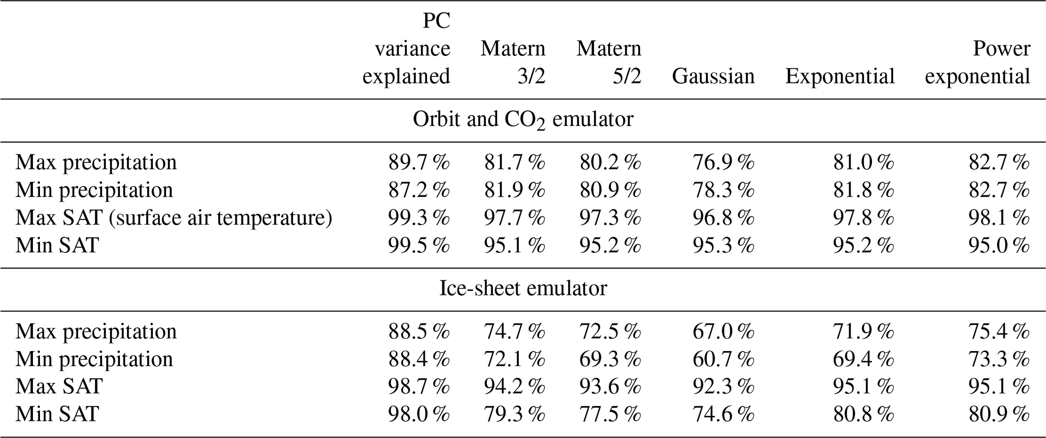
The temperature decompositions explain 94 %–99 % of the ensemble variance, compared to 87 %–90 % for the precipitation decompositions. Under emulation, the variance explained is 81 %–98 % for the temperature fields and 73 %–83 % for precipitation fields. The emulator performance is weaker for precipitation because the low-order components needed to explain much of the ensemble variability are more difficult to emulate.

The power exponential was found to give comparable or better performance compared to the other covariance functions in all eight emulators and was therefore chosen as the default covariance function and used in all analysis that follows.

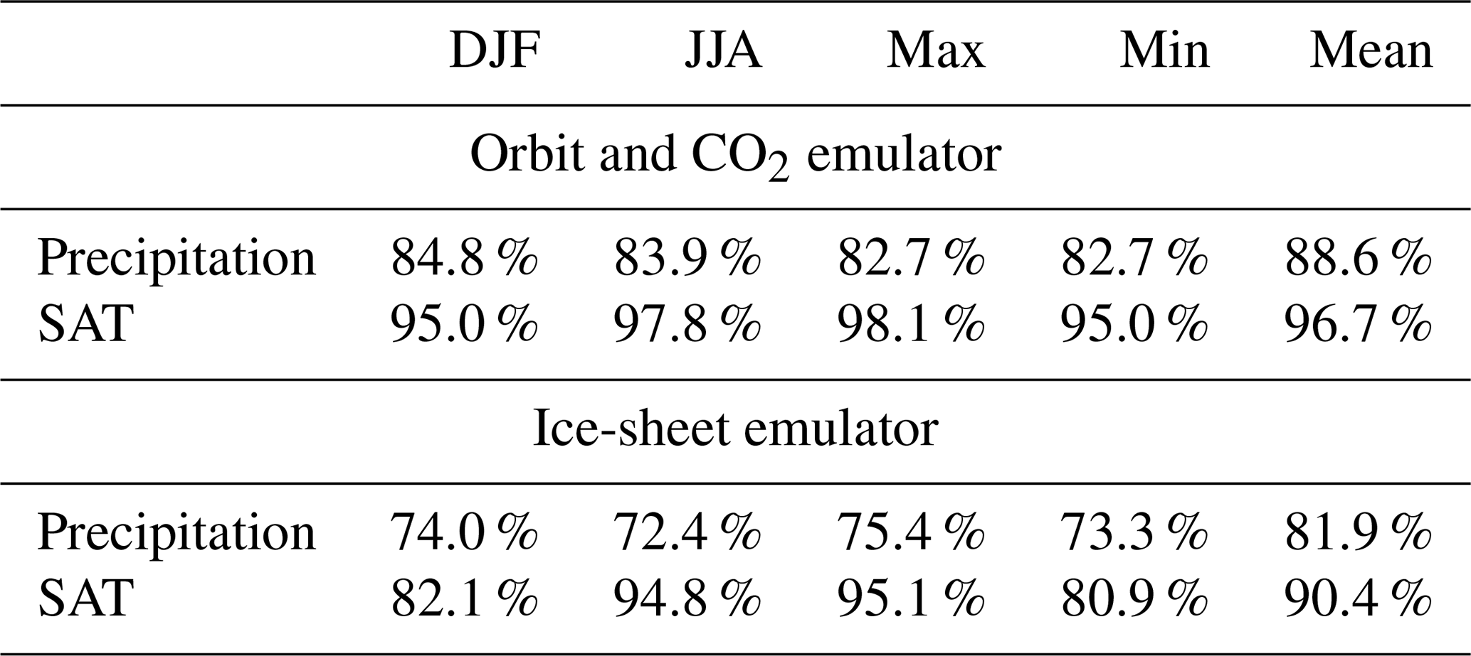
Table 4 summarizes the variance explained under cross-validation of the seasonal and annual average emulators used in the following Sect. 7. DJF (JJA) temperature emulator performance is similar to min (max) temperature emulator performance, suggesting that Northern Hemisphere temperature is more difficult to emulate than Southern Hemisphere temperature, as would be expected for the ice-sheet emulator in particular. The performance of the various seasonal precipitation emulators is similar (82.7 % to 84.8 % for the orbit and CO₂ emulator, 72.4 % to 75.4 % for the ice-sheet emulator), but annual precipitation is easier to emulate than seasonal precipitation (88.6 % for the orbit and CO₂ emulator, 81.9 % for the ice-sheet emulator).

Table 4Seasonal and annual mean emulator performance (as used in Sect. 7), measured by the metric P (Eq. 3, including 10 components). A power exponential covariance is used in all cases. Note that max and min values repeat data from Table 3.

Download Print Version | Download XLSX

The emulators generate a paleoclimate as

where M is the simulation mean field that was subtracted to centre the ensemble before decomposition (Sect. 5). To generate a paleoclimate time series, we therefore require time series of the boundary condition inputs $e,\mathit{\omega },\mathit{\epsilon }{\mathrm{CO}}_{\mathrm{2}}$, and S.

For the orbital parameter inputs, we applied the 5×10⁶-year calculation of Berger and Loutre (1991, 1999). We used CO₂ from Antarctic ice cores for the last 800 000 years (Luethi et al., 2008). Prior to 800 000 BP, and for the entire sea-level record, we used the CO₂ and sea-level reconstructions of Stap et al. (2017). These authors used a zonally averaged energy balance model coupled to a six-level ocean model, a thermodynamic sea-ice model and to one-dimensional mass-balance modules for each of the five major Cenozoic ice sheets (East and West Antarctica, Greenland, Laurentide, and Eurasian). The Stap model is forced with benthic δ¹⁸O records and uses an inversion routine to de-convolve the temperature and ice-volume components of the isotope signal and generate a self-consistent time series of CO₂ and sea level (ice volume).

Figure 2 plots the forcing time series and an illustrative application of the emulator, for which we emulated the time-varying annual mean surface air temperature field and plotted its area-weighted global average through time.

In order to validate the emulators, we performed a series of experiments with Mid-Holocene (MH), Last Glacial Maximum (LGM), Last Interglacial (LIG) and mid-Pliocene warm period (MPWP) CO₂, ice sheets, and orbital forcing. These time slices have been well-studied in Paleo-Modelling Inter-comparison Projects and are well suited to exploring variability driven by all three forcings. The MH and LIG responses are dominantly forced by orbit, while the MPWP is dominantly forced by CO₂ and the LGM by both CO₂ and ice-sheet state.

7.1 Mid-Holocene emulated ensemble

To assist comparison with readily available PMIP2 data (Braconnot et al., 2007), we here emulate seasonal (DJF and JJA) fields rather than seasonal (MAX and MIN) fields, plotted in Fig. 3. Uncertainty is associated with the emulation of the component scores. Gaussian process emulation quantifies this uncertainty by providing a mean prediction and an estimate of the uncertainty associated with that prediction. We generated a 200-member emulation ensemble with MH forcing. The 200 ensemble members differ because we do not assume the mean prediction for the emulated component scores but instead draw randomly from the posterior distributions. In Fig. 3 this ensemble is summarized with mean and standard deviation fields. (We note that for applications in which climate uncertainty is not addressed, it is appropriate to use the mean predictions of principal component scores to generate the best estimate.)

Figure 3PALEO-PGEM emulated ensemble comparison with PMIP2 ocean–atmosphere–vegetation ensemble (Braconnot et al., 2007) for the Mid-Holocene.

Figure 3 (top panels) compares emulated MH surface temperature (anomalies relative to pre-industrial) with the PMIP2 OAV (coupled atmosphere–ocean–vegetation) ensemble. In northern winter DJF, high-latitude warming is apparent in the emulated ensemble mean, although it is of uncertain sign (variability > mean). Cooling is apparent over all other land regions. In northern summer JJA, robust warming is apparent at mid- to high latitudes, while changes in variable signs are apparent in the tropics, with cooling apparent over the Sahel, India, and SE Asia. Each of these features is also found in the PMIP ensemble. The most significant difference is Antarctic cooling of ∼3 ^∘C in PALEO-PGEM, which contrasts with a warming signal in the ensemble mean of PMIP2 (although we note the DJF Antarctic cooling of 0.5 ^∘C was simulated in HadCM3M2). A significant cold Antarctic bias is also apparent during the Last Interglacial (Sect. 7.4). High southern latitudes are poorly modelled by PLASIM-GENIE. The pre-industrial state exhibits a warm Antarctic bias, with greatly understated sea ice, a slow Antarctic Circumpolar Current, and weak, northerly shifted zonal winds (Holden et al., 2016), which are likely associated with the well-known difficulties of resolving Southern Ocean wind stress at low meridional resolution (Tibaldi et al., 1990; Schmittner et al., 2010).

Figure 3 (lower panels) compares emulated MH precipitation with the PMIP2 OAV ensemble. In DJF, significant drying is emulated over central and northwestern South America, southern Africa, eastern Asia, and northern Australia, while wetter conditions are emulated over northeastern South America. In JJA the largest changes are seen as a strengthening of the Asian monsoon precipitation, and significantly wetter conditions are also seen over the Sahel and western South America. These changes all reflect a general agreement with PMIP2.

7.2 Last Glacial Maximum emulated ensemble

We follow the emulated ensemble procedure for the Last Glacial Maximum. Figure 4 (upper panels) compares the emulated Last Glacial Maximum temperatures with the PMIP2 OA (ocean–atmosphere) ensemble. We neglect the OAV LGM ensemble because it has only two simulations. LGM cooling is dominated by cooling of up to ∼40 ^∘C over the Northern Hemisphere glacial ice sheets. The most significant differences are apparent in the emulated uncertainty, which is understated by a factor of roughly 2 relative to PMIP. This is expected because the emulator is built from a single parameterization of PLASIM-GENIE and therefore does not capture uncertain climate sensitivity. We note that by applying the principles of invariant temperature pattern scaling (Tebaldi and Arblaster, 2014), the temperature uncertainties due to neglected climate sensitivity could be approximated by inflating the variance of the principal component scores.

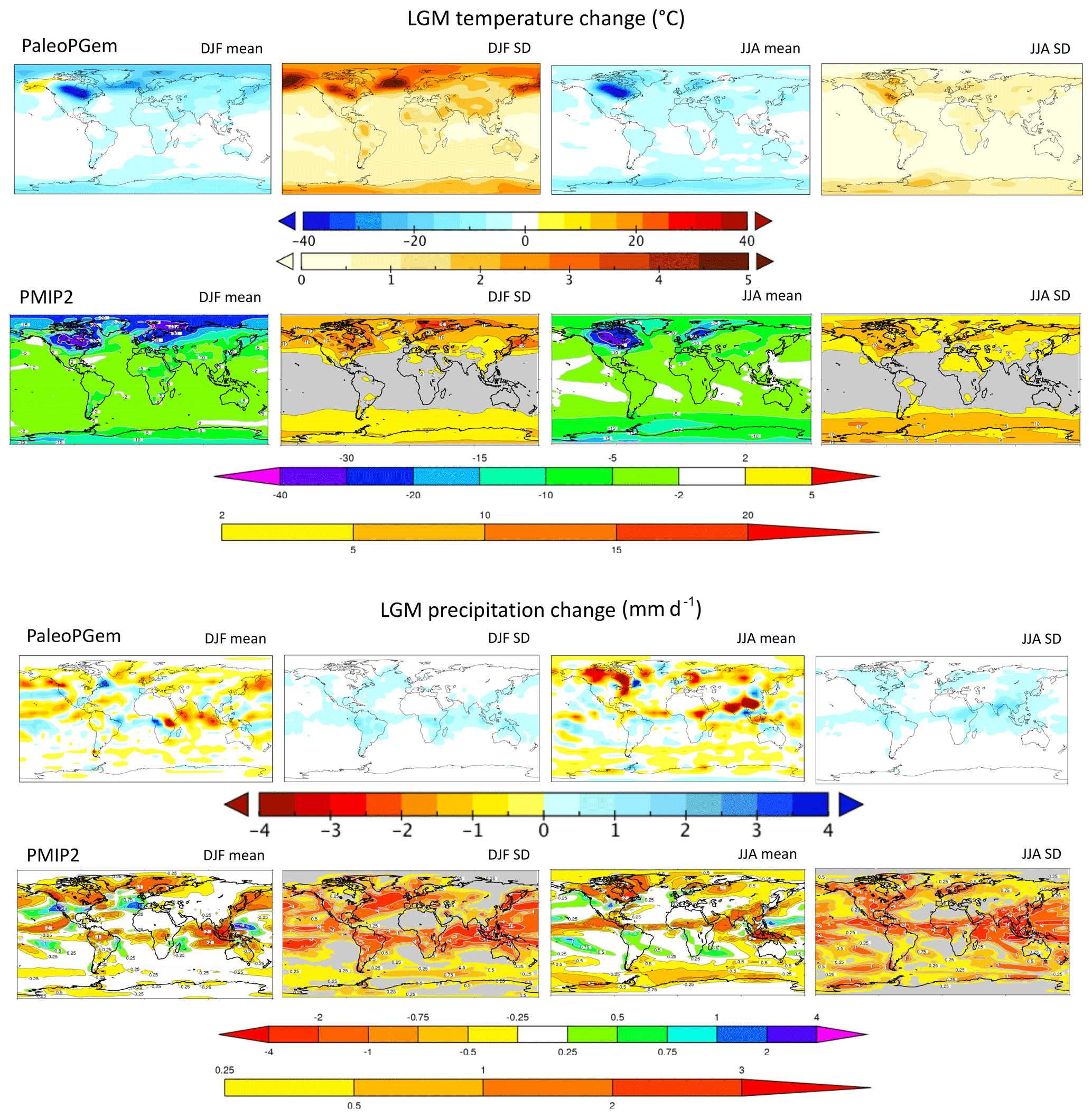
Figure 4PALEO-PGEM emulated ensemble comparison with the PMIP2 ocean–atmosphere ensemble (Braconnot et al., 2007) for the Last Glacial Maximum. Note the different scales for SD temperature. Reduced variance in PALEO-PGEM is due to the understated uncertainty of climate sensitivity, which arises from the neglect of parametric uncertainty.

Figure 4 (lower panels) compares emulated Last Glacial Maximum precipitation with the PMIP2 OA ensemble. In DJF, the drying apparent in central Africa, northern America, and the Amazon are captured by the emulator, while JJA drying at northern latitudes and in the Asian and African monsoon regions and increased precipitation in South America are common to the emulator and the PMIP2 ensemble.

7.5 The mid-Pliocene warm period

The emulated climate of the mid-Pliocene warm period is plotted in Fig. 7. The only emulator forcing is CO₂ increased to 405 ppm, as assumed in the model inter-comparison of Haywood et al. (2013). Ice sheets are fixed at the present day, in contrast to Haywood et al. (2013), where the boundary conditions included a reduced West Antarctic Ice Sheet.

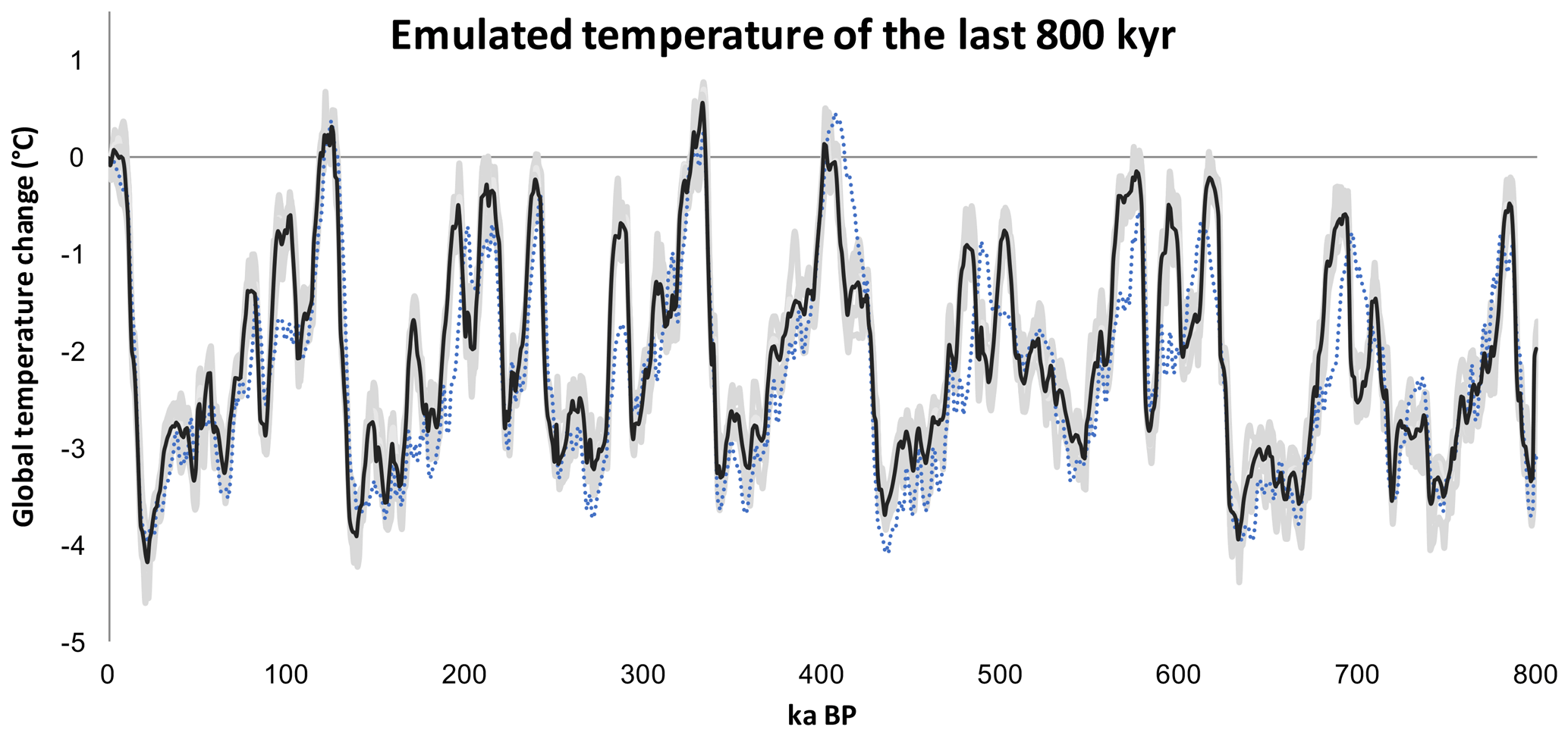
Figure 5Emulated global temperature over the last 800 000 years. An emulator was built 10 times, and the mean prediction time series of each emulator are plotted as grey lines, with the mean of these plotted as the single black line. The blue dotted line is the observationally based reconstruction of Koehler et al. (2010).

Download

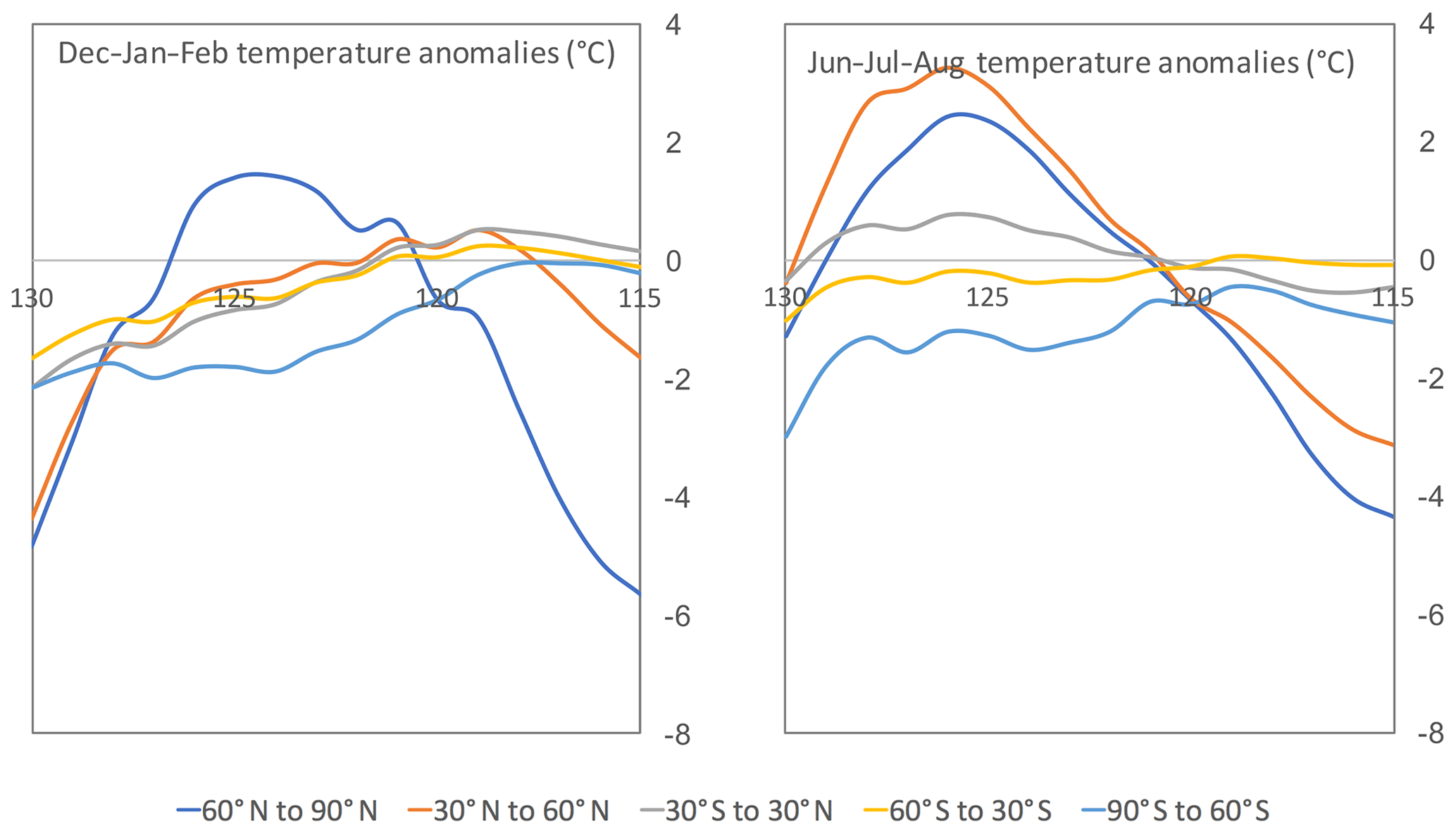
Figure 6Emulated Last Interglacial temperature anomalies with respect to pre-industrial temperatures. An emulator was built 10 times, and the mean prediction time series of each emulator are plotted. Data are provided for December–January–February and June–July–August averaged over five latitude bands; cf. Figs. 2 and 3 of Bakker et al. (2013).

Download

Table 5Last Interglacial peak warming (^∘C) and year of peak warming (BP) compared to the model inter-comparison ±1σ ranges of Bakker et al. (2013). Emulated data are provided for December–January–February and June–July–August, compared to January and July data in the model inter-comparison, and comparisons are provided for five latitude bands.

Download Print Version | Download XLSX

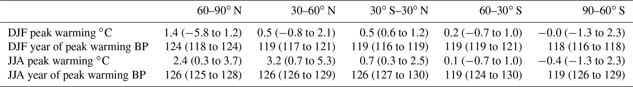
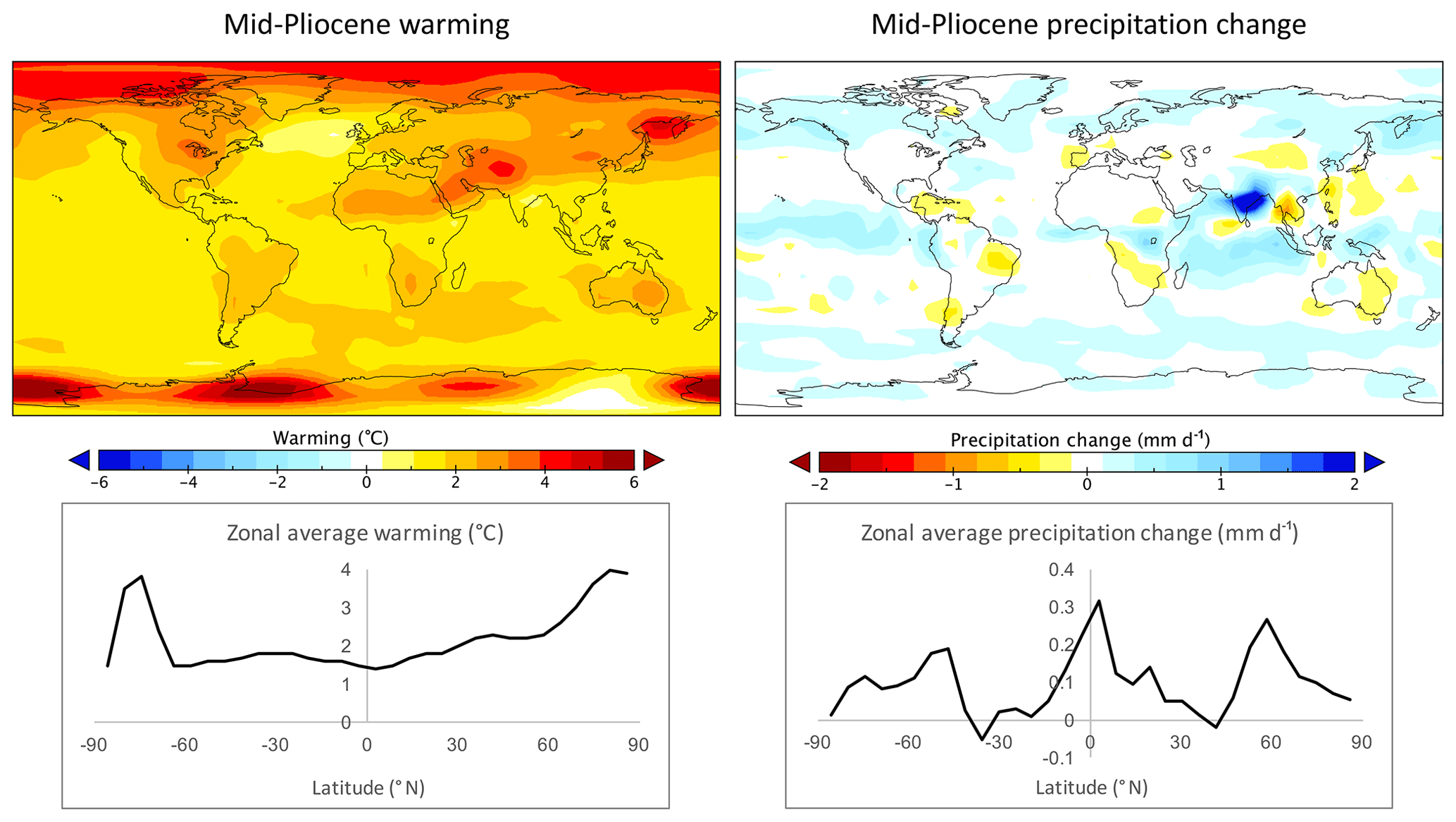
Figure 7Emulated mid-Pliocene temperature and precipitation anomalies with respect to pre-industrial values. The ice-sheet and orbital inputs are set to pre-industrial values, and the emulated change is driven by an assumed CO₂ concentration of 405 ppm.

Ensemble-averaged emulated warming is 1.6±0.2 ^∘C and global precipitation change 0.10±0.01 mm d⁻¹. These compare to multi-model estimates of 1.8 to 3.6 ^∘C and precipitation changes of 0.09 to 0.18 mm d⁻¹ in Experiment 2 (the coupled atmosphere–ocean configuration) of Haywood et al. (2013). Emulated high-latitude warming of ∼4 ^∘C is low-biased, but within the wide multi-model uncertainty range of ∼3 to 14 ^∘C. Similarly, the emulated peak precipitation change of ∼0.3 mm d⁻¹ near the Equator is low-biased, but within the multi-model range of ∼0 to 1.3 mm d⁻¹.

A spatial resolution higher than the native resolution of the underlying climate model may be required for paleo-applications given the scale dependency of many patterns and processes (e.g. Rahbek, 2005), such as scale-dependent climate heterogeneity (Rangel et al., 2018). We address this need by interpolating the low-resolution climate model anomalies onto fine-resolution climatological data. This approach is widely used in climate impact assessment (e.g. Osborn et al., 2016) and has also been applied in paleo-applications in anthropology (Melchionna et al., 2018) and ecology (Rangel et al., 2018).

Downscaling can be performed in any given grid. Here we illustrate downscaling on a global hexagonal grid build on a geodesic dome because it minimizes geographic distortions in shape, area, and distance that are common to map projections. The hexagonal grid is composed of 17 151 quasi equal-area cells of 6918±859 km² whose area variation is not spatially structured.

The four present-day (pre-industrial) emulated bioclimatic variables E were linearly interpolated onto the geodesic grid. All emulations used the mean prediction, and the E1 and E2 emulators were both truncated at 10 principal components. Contemporary observations of the bioclimatic variables C were derived from WorldClim (Hijmans et al., 2005), which provides temperature and precipitation estimates at 1 km² resolution, interpolated from temporally averaged measurements (1950 to 2000) from ∼15 000 to 50 000 weather stations globally (depending upon the variable). The raw emulated climate data E and the difference with observed climatology E0−C are illustrated in Fig. 8.

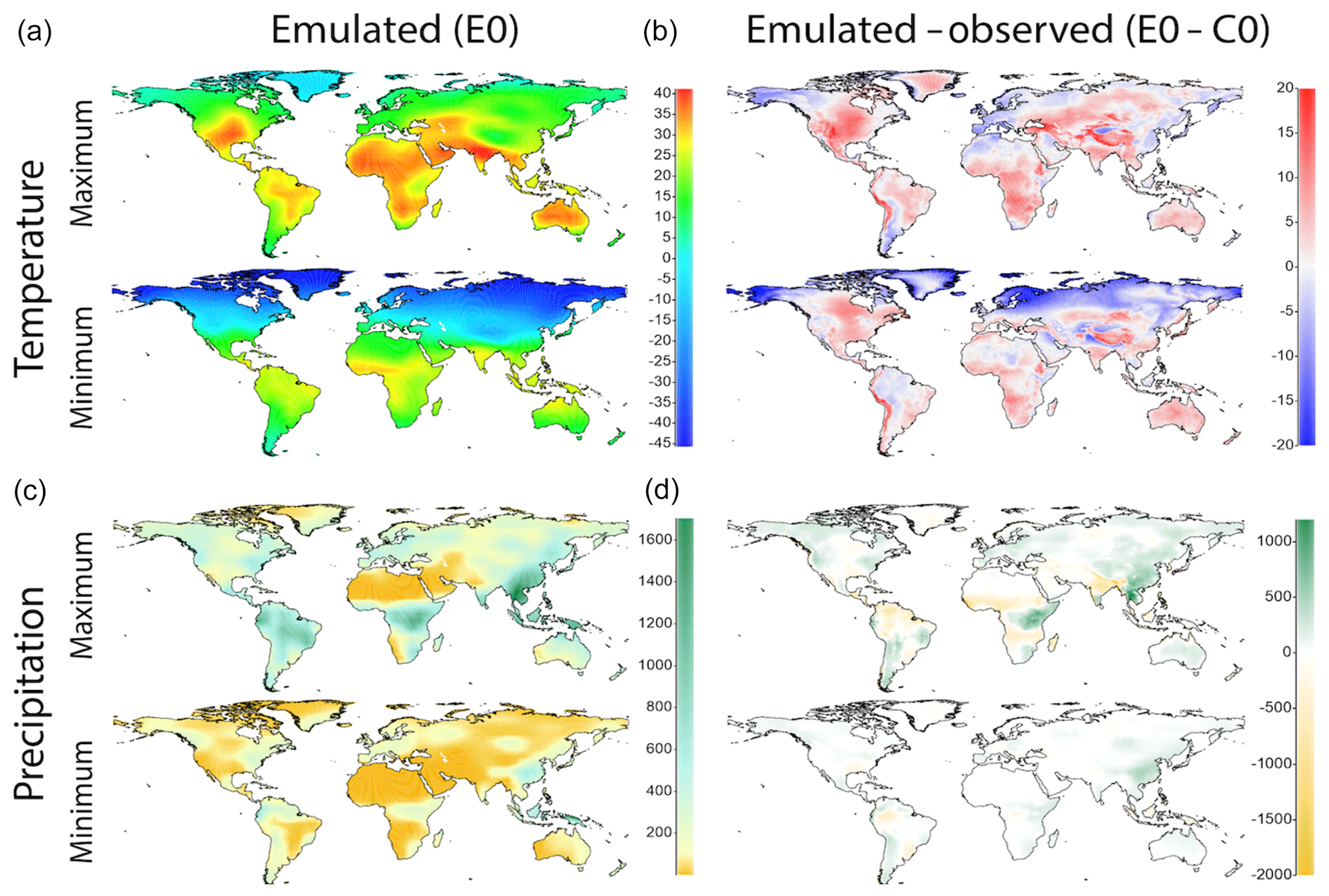
Figure 8Downscaling the emulated climate. Panels (a) and (c) are the pre-industrial emulations of the seasonal bioclimatic variables at native (T21) model resolution, interpolated into the high-resolution grid. Panels (b) and (d) illustrate the differences with respect to high-resolution climatology (Hijmans et al., 2005).

The emulated climatology is reasonable, accepting the low resolution of the underlying climate model. Cold biases are generally confined to northern winter high latitudes. Warm biases are more modest except for the Tibetan Plateau and Andes where the lapse rate cooling in these narrow mountain chains is poorly resolved by the climate model (but corrected for by the downscaling approach described below). Excess precipitation bias is mostly apparent in the (wet-season) monsoon regions. Deserts are generally well resolved in the emulator, a notable exception being the hyper-arid Atacama, which is an orography-driven feature that cannot be captured at low resolution. Conversely, orography-driven precipitation is understated in the Tibetan Plateau. Precipitation is also understated in the Sahel.

We apply anomaly adjustments to derive downscaled emulated climate fields through time Ct. This approach preserves the high-resolution spatial heterogeneity of climatology. In the case of temperature this is straightforward. Emulated anomalies Et−E are interpolated onto the hexagonal grid and applied additively; i.e. $Ct=C\mathrm{0}+\left(Et-E\mathrm{0}\right)$. For precipitation, the situation is more complex. In arid regions that are not well captured by the emulator, a multiplicative anomaly approach is preferable $Ct=C\mathrm{0}\times \left(Et/E\mathrm{0}\right)$, preserving hyper-arid (topographically forced) desert and preventing unphysical negative precipitation when $Et-E\mathrm{0}<\mathrm{0}$. Conversely, in wet regions that are understated by the emulator, a multiplicative anomaly approach can create unphysically high precipitation, but an additive approach ensures a physically reasonable solution. A pragmatic solution to this is to apply an additive precipitation anomaly when E0<C0 and a multiplicative precipitation anomaly when E0>C0. This approach is well-behaved, noting that the additive and multiplicative anomalies are equivalent when E0=C0. Consider, when E0<C0,

and the additive anomaly partially compensates for the low bias in emulated climatological precipitation. Conversely, when E0>C0,

and the multiplicative anomaly partially compensates for the high bias in emulated climatological precipitation.

The present-day climatology and downscaled emulated LGM climate are illustrated in Fig. 9. An animation of the entire 5 000 000-year reconstruction is provided as a Supplement.

PALEO-PGEM is to our knowledge the first attempt to provide a detailed spatio-temporal description of the climate of the entire Pliocene–Pleistocene period. It is essential to understand the main limitations of our modelling framework, discussed below, some of which may induce large errors or uncertainties in specific applications or even rule out certain applications completely. For all practical purposes and for the foreseeable future, substantial uncertainties exist in any paleoclimate reconstruction as a result of incomplete knowledge, computing limitations, and irreducible climatic noise. Ideally, these uncertainties should be quantified in relation to any reconstruction and their implications propagated through the analysis. Our approach provides an estimate of inherent uncertainty derived from the emulation step of the reconstruction and thus underestimates the full uncertainty, but nevertheless in some aspects remains comparable to the uncertainty in state-of-the-art reconstructions of particular periods as measured by the variance across ensembles of PMIP simulations.

Compared to state-of-the-art models, PLASIM-GENIE is a relatively low-resolution, intermediate-complexity climate model. This implies that processes operating at spatial and temporal scales below the native resolution of the climate model cannot be properly represented, although certain aspects of spatial variation are reintroduced in a highly idealized way by the downscaling process. The temporal effects of dynamical processes operating at sub-millennial timescales are further filtered out by the approximation inherent in the emulator construction that the climate is in quasi-equilibrium with the forcing, which is then only resolved at 1000-year time intervals.

Figure 9Downscaled emulated climate. Panels (a) and (c) are the downscaled emulated bioclimatic variables at the Last Glacial Maximum. Panels (b) and (d) are the present-day climatology (Hijmans et al., 2005). Note that downscaled climates are derived by applying emulated anomalies to this present-day climatology. An animation of the complete 5 Ma reconstruction is provided as Supplement.

In applications where (downscaled) time-slice simulations are adequate and are available from higher-complexity models and/or multi-model ensembles (Sect. 7), these would normally be preferable to PALEO-PGEM as errors and biases will generally be smaller, particularly in high latitudes, regions of steep topography, close to coastlines, or in known regions of locally extreme climate. We note that HadCM3 climate simulations (Singarayer et al., 2017), downscaled to 1^∘ resolution are available back to 120 ka (Saupe et al., 2019), which would provide preferable (or supplementary) climate data for applications restricted to this time domain.

The emulator uncertainty captures much of the uncertainty seen in multi-model inter-comparisons (Figs. 3 and 4), but PALEO-PGEM cannot fully represent model uncertainty because it is derived from a single configuration of a single model. Most clearly in this respect, the 90 % uncertainty range of climate sensitivity (3.8±0.6 ^∘C) is understated relative to multi-model estimates of 3.2±1.3 ^∘C (Flato et al., 2013). Some significant biases in spatial patterns are also apparent, most clearly temperature biases in high southern latitudes.

Emulator forcing is limited to orbit, CO₂, and ice sheets. Ice meltwater forcing is not considered, so that millennial variability, especially important in North Atlantic, is neglected. The land–sea mask and orography are held fixed, so that ocean circulation changes driven by changing gateways (e.g. the closing Panama isthmus, with implications for the thermohaline circulation) are neglected and feedbacks driven by changing orography are neglected, especially important in regions of rapid tectonic uplift.

The representation of ice sheets applies Peltier ICE-5G deglaciation ice sheets (Peltier, 2004), assuming a fixed relationship between global sea-level reconstructions (derived from benthic oxygen isotopes) and the spatial form and extent of ice sheets. This approximation neglects the substantial asymmetry between build-up and decay phases of ice sheets and assumes that ice sheets were located similarly in all previous Pliocene–Pleistocene glaciations, which may not have been the case. Particular caution is therefore essential when applying the climate reconstruction at locations near the margins of ice sheets.

We apply a downscaling approach because spatial climate gradients can be critically important for ecosystem dynamics, especially in mountainous regions which are poorly resolved at native climate model resolution (Rangel et al., 2018). The downscaling approximation assumes that the lapse rate within a downscaled grid cell does not change with time, but it does capture the first-order effect of topographic complexity by assuming a constant present-day lapse rate. Similarly, the downscaling cannot capture feedbacks between atmospheric circulation and high-resolution topography, which could alter the patterns of rain shadowing. However, for many applications, it is preferable to neglect this second-order feedback rather than to neglect the first-order effect of a rain shadow that could not be resolved at native climate model resolution (e.g. the Atacama), which downscaling imposes through the baseline climatology. Other simplifications include the implicit assumptions of fixed mountain glaciers and ecotone distributions. In short, the high-resolution reconstructions should not be interpreted as a faithful reconstruction of high-resolution climate but should serve to introduce a more realistic degree of spatial variability.

The Supplement contains all of the files needed to build the emulators. PALEO-PGEMv1.0_5M_1Ka.mp4 is an animation of the four bioclimatic variables over 5Ma. PALEO-PGEMv1.0.R is the R code to build and run the emulators. A series of files are inputs to the R code. These are ensemble.dat (the ensemble input design for the BC1/BC2 ensembles), 5000_1000_forcing.dat (time series forcing for 5 Ma at 1 kyr intervals), MH_forcing.dat (Mid-Holocene ensemble forcing), LGM_forcing.dat (Last Glacial Maximum forcing), and area.dat (grid cell areas for area weighting). Two subdirectories contain the simulation data: data (outputs of the BC1 PLASIM-GENIE ensemble) and icedata (outputs of the BC2 PLASIM-GENIE ensemble). Supporting data are included in two spreadsheets: ensemble (supporting calculations for the ensemble design) and 5000ka_forcing (supporting calculations for the time series forcing). PALEO-PGEMv1.0.R was saved with settings to emulate DJF temperature and produce a 5 Ma time series using the GP mean prediction (no emulator uncertainty), 10 principal components, and a power exponential covariance function. Each of these settings can be changed as documented in the code. The code outputs the area-weighted average to screen and three data sets to file: emul.dat (the full spatio-temporal output), mean.dat, and SD.dat (the mean and standard deviation of the emulated fields, most relevant when code is set to generate an ensemble, e.g. with MH or LGM forcing).

The supplement related to this article is available online at: https://doi.org/10.5194/gmd-12-5137-2019-supplement.

PBH, NRE, and TFR developed the concept. PBH performed the PLASIM-GENIE simulations, using boundary conditions developed by GTT. PBH and RDW developed the GP emulators. TFR and EBP developed the downscaling, with advice from PBH and NRE. PBH wrote the paper with contributions from all authors.

The authors declare that they have no conflict of interest.

Philip B. Holden and Neil R. Edwards were funded by NERC (grant no. NE/P015093/1). Elisa B. Pereira is supported by a doctorate fellowship from Coordenação de Aperfeiçoamento de Pessoal de Nível Superior – Brasil (CAPES) – Finance Code 001.

This paper was edited by Didier Roche and reviewed by Michel Crucifix and one anonymous referee.