Algorithmic differentiation (AD) is a mathematical theory that describes how the computation of derivatives in a computer program can be automatized. It was developed in the early 1980s and rediscovered several times since then. The most well-known resource is the book of Griewank and Walther (2008). A useful first introduction is given by Neidinger (2010).

For the purpose of computing the derivative of a program, it is considered as a sequence of simple elemental (or intrinsic) functions including the sine, cosine, multiplication, division, and addition. The approach of AD considers the given program as a composition of elemental functions and, by applying the chain rule, computes its directional derivative by accumulating the derivatives of each elemental function within the program code. It is important to stress that AD does not generate a generalized representation of the derivative of the computer program. Instead, AD computes the derivatives alongside the execution path. The path might change due to conditional instructions within the code.

As an example, assume the computer program to be differentiated is given by

where $a,b,c,d$ are the input variables and w is the output. This program can now be split into elemental functions which yield the intermediate steps t₁, t₂ required by AD as follows:

For the application of the chain rule the Jacobian matrix has to be computed for each of these intermediate steps with respect to all input variables, which is quite simple; e.g., for $t_{\mathrm{1}}=t_{\mathrm{1}}(a,b,c,d)=a+b$ the matrix is $(\mathrm{1},\mathrm{1},\mathrm{0},\mathrm{0})$ since $\frac{\partial t_{\mathrm{1}}}{\partial a}=\frac{\partial t_{\mathrm{1}}}{\partial b}=\mathrm{1}$ and $\frac{\partial t_{\mathrm{1}}}{\partial c}=\frac{\partial t_{\mathrm{1}}}{\partial d}=\mathrm{0}$. However, for notational convenience it is common to drop the indication of the formal dependence of the elemental function t₁ and its derivatives on the input parameters c, d since they are unchanged in t₁. In order to compute the directional derivative, the Jacobian matrix is multiplied with the desired direction $(\dot{a},\dot{b},\dot{c},\dot{d}{)}^T$, where the dot notation is used in the AD theory to describe the corresponding derivative direction of a variable. Applying this process to the full procedure Eq. (2), the result is

since, e.g.,

where we again neglected the formal dependency of t₁ on c and d. By computing the corresponding directional derivative statements in procedure Eq. (3) alongside the original statements in procedure Eq. (2), the directional derivative is computed for the whole computer program Eq. (1). Note that the choices $(\dot{a},\dot{b},\dot{c},\dot{d})=(\mathrm{1},\mathrm{0},\mathrm{0},\mathrm{0})$ and $(\dot{a},\dot{b},\dot{c},\dot{d})=(\mathrm{0},\mathrm{1},\mathrm{0},\mathrm{0})$ for the input directions for the AD computation results in the computation of the partial derivatives $\frac{\partial w}{\partial a}$ and $\frac{\partial w}{\partial b}$.

The example shows the application of the forward AD mode on a simple computer program. The general theory of AD assumes that the elemental functions are evaluated at argument values where they are differentiable in a neighborhood of the argument value. Actually, many common elemental functions are differentiable everywhere as, e.g., addition or multiplication, but there are elemental functions which are differentiable except at some critical points. Examples for elemental functions with a critical point are square root, absolute value, and division, which are not differentiable at the origin. How these difficulties are treated mainly depends on the AD tool. The AD tool CoDiPack used in this study provides the preprocessor option CODI_CheckExpressionArguments to throw an exception if such a critical point is encountered. In any case, the exact derivative of each elemental function, at least apart from the critical points, may be written down explicitly. Note that conditional instructions (e.g., if-else switches) do not pose problems, since they only alter the program path, i.e., the specific sequence of the elemental instructions that are executed. Since the whole computer program is a composition of the differentiable elemental operations, the chain rule states that also the whole program is differentiable (apart from the critical points). Moreover, if the program is represented by the function $\widehat{f}:{\mathbb{R}}^n\to {\mathbb{R}}^m$, the so-called forward mode of AD computes

In Eq. (5), $\frac{\mathrm{d}\widehat{f}}{\mathrm{d}x}\left(x\right)$ is the Jacobian of the full program at state x, vector $\dot{x}$ is the direction for which the program derivative is desired along the computational path and the variable x subsumes all input variables. In the notation of Sect. 1, we have $x=\left(y,\mathit{\eta }\right)$, i.e., x contains the cloud model and thermodynamic variables y together with the inherent parameters η. In this terminology, an inherent parameter of the (cloud) model is also now considered as a parameter if this parameter is to be investigated.

Equation (5) just states which result is computed by the forward mode of AD and not how it is computed. The evaluation of the derivative is done alongside the primal computation of $\widehat{f}\left(x\right)$ by applying Eq. (5) to each elemental operation as in the above example, i.e., the full Jacobian is never computed explicitly but accumulated by considering each code statement individually.

The second operation mode of AD is called the reverse AD mode. As will become clear, the reverse mode can be introduced by multiplying an adjoint direction from the left side to the derivative representation of the computer program, instead of multiplying a derivative direction from the right as in Eq. (5). This yields the general equation ${\stackrel{\mathrm{‾}}{x}}^T={\stackrel{\mathrm{‾}}{z}}^T\frac{\mathrm{d}\widehat{f}}{\mathrm{d}x}\left(x\right)$. The standard AD notation for the adjoint of a variable v is the bar notation $\stackrel{\mathrm{‾}}{v}$ and may be thought of as containing the immediate derivative of the current statement with respect to the particular variable.

As an example, for the statement $w=t_{\mathrm{1}}\cdot t_{\mathrm{2}}$, the AD reverse mode evaluation is

The information flow in Eq. (6) is reversed for the adjoint variables: the input variable is $\stackrel{\mathrm{‾}}{w}$, while ${\stackrel{\mathrm{‾}}{t}}_{\mathrm{1}}$ and ${\stackrel{\mathrm{‾}}{t}}_{\mathrm{2}}$ are output variables. Because of this reversal of the information flow, all reverse AD statements need to be evaluated in reverse order. The reverse of the last statement of the program code $\widehat{f}$ will be evaluated first, the second to last statement as second, and so on. The reverse AD procedure for the example procedure Eq. (2) is then

As discussed above, the statements from procedure Eq. (2) are now handled in reverse order. The values $\stackrel{\mathrm{‾}}{a}$, $\stackrel{\mathrm{‾}}{b}$, $\stackrel{\mathrm{‾}}{c}$, and $\stackrel{\mathrm{‾}}{d}$ contain the derivatives of w with respect to themselves. Taking $\stackrel{\mathrm{‾}}{d}$ as an example, according to the chain rule this is

and the value of t₁ is taken from the primal evaluation of the program. By choosing $\stackrel{\mathrm{‾}}{w}=\mathrm{1}$ as input for the reverse AD mode, the adjoint variable $\stackrel{\mathrm{‾}}{d}$ contains the derivative of procedure Eq. (2) with respect to the input d.

The example, Eq. (7), shows the application of the reverse AD mode on a simple computer program. According to the general theory of AD, given a computer program which can be represented by the function $\widehat{f}:{\mathbb{R}}^n\to {\mathbb{R}}^m$, the reverse AD mode computes

where, again, $\frac{\mathrm{d}\widehat{f}}{\mathrm{d}x}\left(x\right)$ denotes the Jacobian of $\widehat{f}$ and ${\left[\frac{\mathrm{d}\widehat{f}}{\mathrm{d}x}\left(x\right)\right]}^T$ its transpose, while $\stackrel{\mathrm{‾}}{z}$ represents the desired direction for the derivative. Eq. (9) again just states the result that is computed by the reverse mode of AD and not how it is computed. The actual evaluation of the derivative is done without forming the Jacobian and instead by storing information during the primal computation of $\widehat{f}\left(x\right)$. Afterwards, a reverse sweep over the stored information is performed. This reverse sweep applies a slightly modified version of Eq. (9) to each elemental function as in the above example.

Both operation modes of AD are connected via the discrete adjoint operator. Let $\langle \cdot ,\cdot {\rangle }_n$ and $\langle \cdot ,\cdot {\rangle }_m$ denote the Euclidian scalar products in ℝⁿ and ℝ^m, respectively. We now select an arbitrary direction $\stackrel{\mathrm{‾}}{z}\in {\mathbb{R}}^m$, which we apply to the result of the forward mode. This yields the equality

by shifting the Jacobian matrix of $\widehat{f}$ to the left side of the scalar product. This shows that the reverse mode is the discrete adjoint of the forward mode (see, e.g., Kalnay, 2003, for the use of adjoint models in atmospheric data assimilation).

The advantage of the reverse mode becomes clear if we assume that we want to compute the full gradient of a function $\widehat{f}:{\mathbb{R}}^n\to {\mathbb{R}}^m$. In the case of m=1, i.e., a computer program with n input and a single output variable, the full gradient $\frac{\mathrm{d}\widehat{f}}{\mathrm{d}x}\left(x\right)$ is a matrix with n columns and one row; hence its transpose is a matrix with n rows and a single column. Since m=1, the direction $\stackrel{\mathrm{‾}}{z}$ is a vector with a single entry. Consequently, we obtain the result $\stackrel{\mathrm{‾}}{x}$ by computing Eq. (9) exactly once with the single input $\stackrel{\mathrm{‾}}{z}=\left(\mathrm{1}\right)\in {\mathbb{R}}^{\mathrm{1}}$. Using the forward mode of AD, we infer from Eq. (5) that the computation of the full gradient requires n subsequent computations with the choices $\dot{x}=e_{\mathrm{1}},\dot{x}=e_{\mathrm{2}},\mathrm{\dots },\dot{x}=e_n$, and e_i∈ℝⁿ denotes the ith unit vector. If n is large, these n subsequent computations require much more computational effort than a single (but slightly more costly) computation using the reverse mode of AD.

In contrast, if n=1, i.e., the computer program has a single input and m output variables, the forward mode of AD computes the full derivative with a single computation by choosing the 1×1 matrix $\dot{x}=\left(\mathrm{1}\right)$ as the input direction, whereas the reverse mode needs m computations, being costly for large values of m.

An alternative approach to compute the derivative of $\widehat{f}:{\mathbb{R}}^n\to {\mathbb{R}}^m$ in the direction d∈ℝⁿ is to apply the finite difference approach

with a (small) step size t>0, requiring two evaluations of the program $\widehat{f}$. Instead of the approximation Eq. (11), one could alternatively choose a finite difference approximation of a higher order (e.g., Grossmann and Roos, 2007), but these typically need even more program evaluations. In contrast to AD, the finite difference approach requires the choice and tuning of the step size t>0 to achieve the desired accuracy of the derivative. Moreover, the optimal value of the step size will in general depend on the selected direction d and the state x (see Elizondo et al., 2002, for a comparison with AD). These issues render the finite difference approach as quite unattractive but due to its simplicity it is often used, accepting all drawbacks of the method.

If $\widehat{f}$ is a linear function, then an arbitrary step size t can be chosen for all directions. For non-linear functions, t should be as small as possible to achieve the desired accuracy but large enough to avoid cancellation errors due to the difference in Eq. (11). AD has the advantage of not having to choose and tune a step size. Since the derivative of each elemental function is known exactly and AD applies the chain rule, the computed derivatives are accurate up to machine precision (Griewank et al., 2012).

Moreover, using the reverse mode for computing the full gradient in the case of only a small number of output variables, AD has the potential of being several times faster compared to using finite difference approximations.

AD is introduced into computer programs mostly in two ways: either through operator overloading or through source transformation. For C++, the majority of tools (as listed at http://www.autodiff.org, last access: 23 October 2019) use the operator overloading approach which is also used by the AD tool CoDiPack (Sagebaum et al., 2017a) developed by the authors from the Scientific Computing group in Kaiserslautern and employed in this study. CoDiPack uses expression templates to reduce the amount of required information for the reverse AD mode. The data layout of the information is such that a minimal memory footprint is required and caching strategies of the processors can be applied. The general focus of CoDiPack is its application in high performance computing environments which was successfully demonstrated in Sagebaum et al. (2017b) and Albring et al. (2016).

The source transformation approach is mostly used in Fortran source codes. Here, the code is parsed and new code is generated which adds the additional statements for the forward or reverse AD mode. Tapenade (e.g., Hascoët and Pascual, 2013) is the most widespread tool for source transformations in Fortran. It is written in Java and supports nearly all features of older Fortran standards. Support for more modern features in newer Fortran versions is an ongoing development.

In general AD can be applied to any computer program. After an initial effort, the derivative computations can be automatized in the sense that every change in the code will immediately affect the primal computation and also the derivative evaluation. How much time the initial effort requires depends strongly on the code and which AD tool is applied. A general effort at analyzing software and detecting problematic code constructs is done in Hück et al. (2015). In general, operator overloading tools are usually quite easy to introduce into a code if it is well written and there is a distinct place where the computation type of the program can be defined. Source transformation usually requires much greater effort. In both cases an early introduction of AD into the code reveals incorrect implementation assumptions and yields a cleaner code.

As an application for AD, we consider a slightly generalized one-moment scheme for warm cloud microphysics, i.e., liquid clouds without ice, within a zero-dimensional air parcel framework. One-moment schemes are designed to predict the temporal evolution of the mass of non-sedimenting cloud droplets, rain drops, and water vapor, i.e., the mixing ratios $q_{\mathrm{c}}=\frac{M_{\mathrm{c}}}{M_{\mathrm{a}}}$, $q_{\mathrm{r}}=\frac{M_{\mathrm{r}}}{M_{\mathrm{a}}}$, and $q_{\mathrm{v}}=\frac{M_{\mathrm{v}}}{M_{\mathrm{a}}}$ where M_c is the mass of cloud droplets, M_r the mass of rain drops, M_v the mass of water vapor, and M_a the mass of dry air. One-moment schemes have a long history and are governed by the classical partitioning of the droplet spectrum into non-sedimenting cloud droplets and larger rain drops, which fall due to the gravitational acceleration (Kessler, 1969). Although these schemes remain the default choice in many computational models, for example, the operational numerical weather forecast models IFS (ECMWF, 2017), run by the European Center for Medium Range Weather Forecast (ECMWF), and COSMO (Doms et al., 2011), run by the German Weather Service (DWD), much consensus exists that two-moment schemes are in general more accurate (Igel et al., 2015). The difference between a one-moment and a two-moment scheme is that the two-moment scheme not only predicts the evolution of the mass mixing ratios but also the corresponding number concentrations.

The one-moment warm cloud schemes of the IFS and the COSMO model may be written in generic form as (see Rosemeier et al., 2018; Porz et al., 2018)

with the coefficients $c,a_{\mathrm{1}},a_{\mathrm{2}},e_{\mathrm{1}},e_{\mathrm{2}},d$, the exponents $\mathit{\gamma },{\mathit{\beta }}_{\mathrm{c}},{\mathit{\beta }}_{\mathrm{r}},{\mathit{\delta }}_{\mathrm{1}},{\mathit{\delta }}_{\mathrm{2}},\mathit{\zeta }$ and the saturation ratio $S=\frac{p_{\mathrm{v}}}{p_{\mathrm{sat}}}$, comparing the partial pressure p_v of water vapor to the saturation vapor pressure p_sat over a flat surface of water. The scheme includes the following processes:

• i.

  condensational growth of cloud droplets;

• ii.

  autoconversion, describing the formation of rain drops by colliding cloud droplets;

• iii.

  accretion, describing the collection of cloud droplets by falling rain drops;

• iv.

  evaporation of rain drops;

• v.

  sedimentation of rain drops out of the grid box.

The term B subsumes the flux of rain drops falling from above into the considered grid box. The splitting of the evaporation term in Eq. (12d) is due to the appearance of the ventilation factor in the diffusional growth equation for the rain drops, taking a non-uniform distribution of water vapor around the falling rain drop into account.

The major differences of Eq. (12) from the actual scheme in the operational model are the formulations of the sedimentation process as a sum of the incoming and outgoing fluxes B and $d{q}_{\mathrm{r}}^{\mathit{\zeta }}$, and the use of an explicit condensation term, which is usually circumvented by employing a saturation adjustment scheme (Asai, 1965; McDonald, 1963; Langlois, 1973; Soong and Ogura, 1973; Kogan and Martin, 1994). Note that the values of the coefficients may also depend on the environmental conditions. Also note that the formulation in Eq. (12) does not contain a term for the activation of new cloud droplets. Within the operational models, the activation of cloud droplets is done with the help of the saturation adjustment, where the excess water vapor is converted into mass of cloud droplets, thus always activating the maximal number if not restricted otherwise.

After choosing an appropriate set of coefficients and exponents, Eq. (12) represent a cloud scheme for a warm cloud in the spirit of Kessler, although not every choice of parameters yields a physically meaningful scheme. Apart from the condensation term, the parameterizations of the other processes are not based on purely physical reasoning. Rather the structure of the terms represent in some sense ad hoc formulations and approximations, but may also be motivated in the sense of population dynamics. The values of the coefficients and the exponents are usually obtained by fitting to observational data or results of detailed models (e.g., Khairoutdinov and Kogan, 2000). In any case, the precise values of the coefficients and the exponents are uncertain to some degree.

For simplicity, we consider the cloud scheme Eq. (12) within an adiabatic air parcel, providing a natural framework to start with in the development of cloud schemes. The closure of Eq. (12) is given by the evolution equations for pressure p and temperature T:

where g denotes the gravitational acceleration, $\stackrel{\mathrm{‾}}{R}=R_{\mathrm{a}}\left(\mathrm{1}+\frac{\mathrm{1}-\mathit{\epsilon }}{\mathit{\epsilon }}\frac{q_{\mathrm{v}}}{\mathrm{1}+q_{\mathrm{v}}}\right)$ the gas constant for moist air, R_a the gas constant for dry air, R_v the gas constant for water vapor, and $\mathit{\epsilon }=\frac{R_{\mathrm{a}}}{R_{\mathrm{v}}}$ the quotient of the gas constants of dry air and water vapor, w the vertical velocity and L the latent heat of vaporization. The coefficient c of the condensation is given by

with ρ_l the density of water, N_c an assumed constant number concentration of the cloud droplets, and the thermodynamic correction (Howell factor)

for the condensational growth of a cloud droplet. In Eq. (15), K denotes the thermal conductivity of dry air and D the diffusivity of water vapor in air. Note that the choice of a fixed constant cloud droplet number N_c in Eq. (14) is motivated by the default Kessler-type warm cloud scheme of the IFS model (ECMWF, 2017).

Using the notation introduced in Sect. 1, the combined discretization of the governing Eqs. (12) and (13) represents the (mathematical) function $f=f(y,\mathit{\eta })$, taking the values of the foregoing time step

together with the parameters

to compute the state of the system at the new time level, i.e., computing $z=f(y,\mathit{\eta })$. Implementing f yields the function $\widehat{f}$, from which AD can compute the derivatives with respect to the parameters η.

We implemented the air parcel model in C++ and discretized the ordinary differential equations using the classical explicit Runge–Kutta method of order 4 (Hairer et al., 1993), although any other method could be used as well. We chose the values of the parameters according to the warm rain scheme used in the operational forecast model IFS (ECMWF, 2017). In this case, all exponents are independent of the environmental conditions and only the coefficients e₁, e₂ of the evaporation depend on the environmental conditions. Table 1 collects the values of the constant coefficients and exponents together with the values of e₁, e₂ at pressure 850 hPa and temperature 270 K. Note that e₁, e₂ vary only weakly with pressure and temperature. Prior to each time step, we compute the values of the parameters e₁, e₂ for the cloud model using the environmental values of pressure and temperature from the old time step. This fixes the values of the parameters for the call to the function $\widehat{f}$, computing numerically a single time step of the governing Eqs. (12) and (13). Using AD, we compute the derivative of the implemented code $\widehat{f}$ with respect to the parameters Eq. (17) at the current time step.

Table 1Values of the coefficients and exponents used for the cloud scheme. All coefficients except for e₁, e₂ are independent of environmental pressure and temperature. The values for the exponents are exact; the values for the coefficients are rounded to three digits. The coefficient values displayed for e₁, e₂ are for environmental pressure 850 hPa and temperature 270 K.

Download Print Version | Download XLSX

In the following, we always assume a constant vertical velocity w, the initial environmental conditions 270 K and 850 hPa, the constant cloud droplet number density ρN_c=50 cm⁻³ (as suggested in ECMWF, 2017 over ocean), no fall of rain drops from above B=0 s⁻¹, and the constant time step Δt=0.01 s. To arrive at a meaningful sedimentation rate, we adopt the assumption of constant terminal velocity of the rain drops from ECMWF (2017) and assume an air parcel with height h=1000 m.

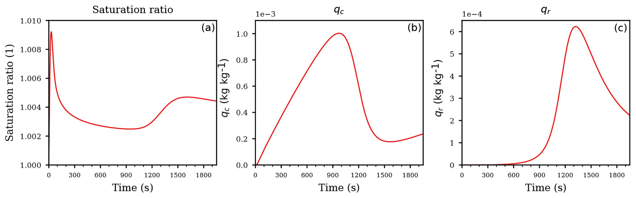
Figure 1Temporal evolution of the saturation ratio S (a), the cloud droplet mixing ratio q_c (b), and the rain drop mixing ratio q_r (c) for the ascending air parcel with no pre-existing clouds.

Download

4.1 Cloud formation in updraft

As the first example we consider an updraft velocity w=1 m s⁻¹, the initial conditions

$$\begin{array}{}\text{(18)}& \left(q_{\mathrm{c}}\left(\mathrm{0}\right),q_{\mathrm{r}}\left(\mathrm{0}\right)\right)=\left({\mathrm{10}}^{-\mathrm{10}}\mathrm{kg}{\mathrm{kg}}^{-\mathrm{1}},\mathrm{0}\mathrm{kg}{\mathrm{kg}}^{-\mathrm{1}}\right)\end{array}$$

for the mixing ratios, and S(0)=1 for the saturation ratio and integrate the governing equations for 1950 s. The reason of not choosing q_c(0)=0 kg kg⁻¹ is that Eq. (12a) needs a non-zero initial value to allow for a non-constant and non-zero solution. Physically, this reflects the fact that the cloud scheme Eq. (12) does not include a precise activation mechanism which predicts the number of activated cloud droplets as a function of saturation ratio. Such a mechanism is not included in the operational model due to its usage of a saturation adjustment scheme (e.g., Kogan and Martin, 1994).

Figure 1a, b, and c show, respectively, the temporal evolution of the saturation ratio S, the cloud droplet mixing ratio q_c, and the rain drop mixing ratio q_r. Apparently, the saturation ratio increases initially due to adiabatic cooling, until cloud droplet mass increased enough to balance the source for the saturation ratio from the adiabatic cooling by the diffusional growth of the cloud droplets. Since autoconversion is the only process for forming rain, its formation starts after enough cloud droplet mass is available. The time interval between 900 and 1200 s is a transition region, where the influence of autoconversion decreases while the influence of accretion increases, i.e., falling rain drops start to effectively collect cloud droplets and consequently increase the rain drop mass mixing ratio q_r. This may also be seen directly from the model Eq. (12): accretion is modeled as $a_{\mathrm{2}}{q}_{\mathrm{c}}^{{\mathit{\beta }}_{\mathrm{c}}}{q}_{\mathrm{r}}^{{\mathit{\beta }}_{\mathrm{r}}}$, hence an increase of rain drop mass directly increases the influence of this process and the further decrease in cloud droplet mass may be attributed to accretion. At about 1200 s the saturation ratio starts to increase again, since the decreasing cloud droplet mass diminishes the sink for water vapor due to its condensational growth. Note that, according to Eq. (12c), the evaporation term is inactive for supersaturated conditions with S≥1.

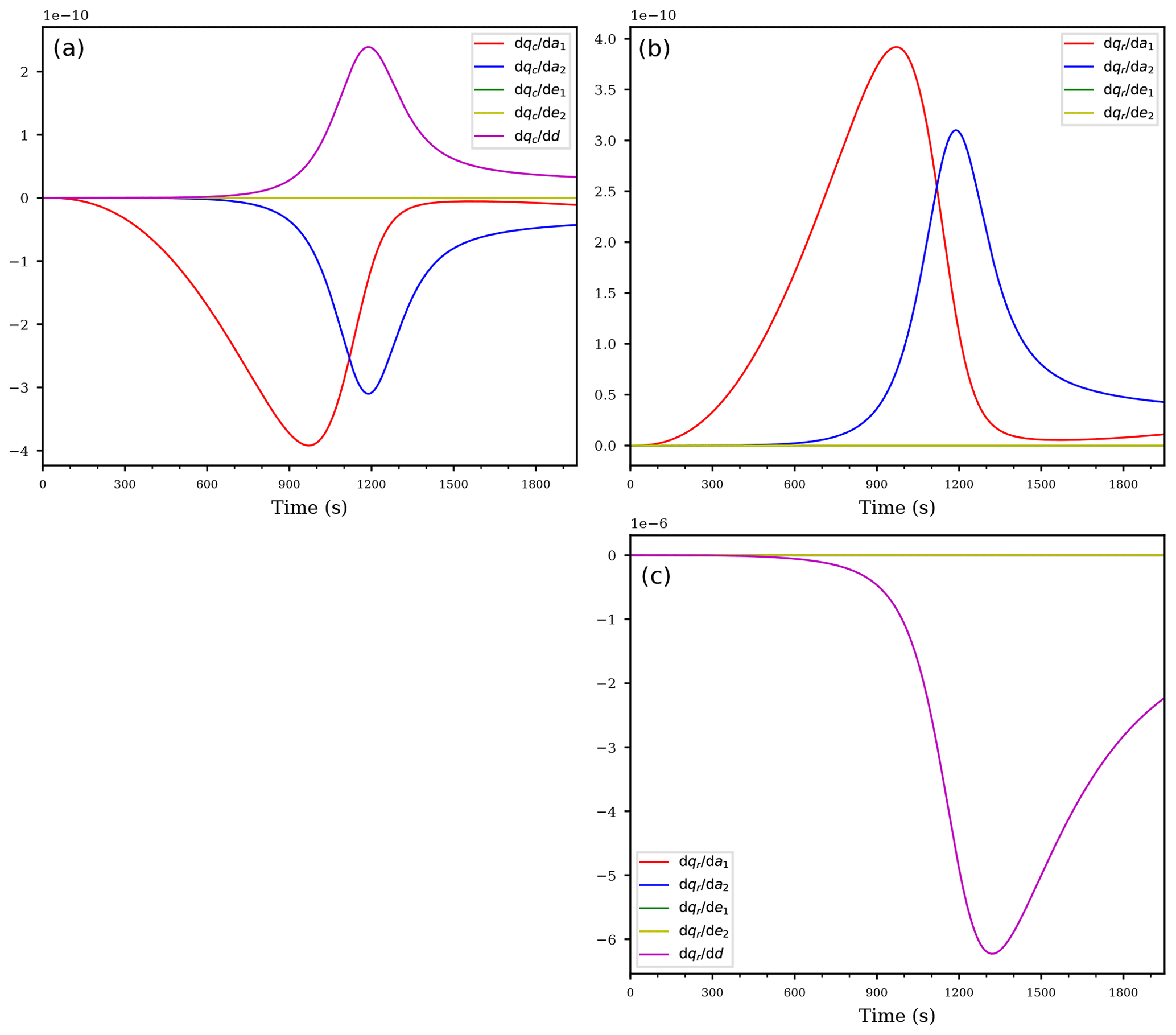
Figure 2Temporal evolution of the derivatives of the cloud droplet mixing ratio q_c (a) and the derivatives of the rain drop mixing ratio q_r (b) and (c) with respect to the coefficients. Panel (b) shows the derivatives of the rain drop mixing ratio q_r with respect to the coefficients but without the derivative $\frac{\partial q_{\mathrm{r}}}{\partial d}$ with respect to the sedimentation coefficient; the panel (c) shows the derivatives of q_r including the derivative with respect to the sedimentation coefficient d (purple curve). All panels correspond to the first case of an ascending air parcel with no pre-existing clouds.

Download

The derivatives of the mixing ratios with respect to the coefficients are shown in Fig. 2, whereas Fig. 3 shows the derivatives with respect to the exponents. As Fig. 2a shows, the coefficient with the largest sensitivity to the cloud droplet mass q_c up to about 1000 s is the coefficient a₁ for autoconversion (red curve). The large sensitivity during the initial stage of the cloud evolution implies that the main loss of cloud droplet mass can be attributed to the autoconversion process, rendering the autoconversion rate a critical parameter. Given that autoconversion is the only process for producing rain drops out of the cloud droplets, this result may be anticipated. The negative value of the derivative $\frac{\partial q_{\mathrm{c}}}{\partial a_{\mathrm{1}}}$ indicates a decrease in q_c if the value of a₁ is increased by a small amount, i.e., a larger autoconversion rate results in a faster decrease of the cloud droplet mass. The transition region between 900 and 1200 s, where the influence of autoconversion decreases and accretion increases, is also clearly visible as a decreasing magnitude of $\frac{\partial q_{\mathrm{c}}}{\partial a_{\mathrm{1}}}$ and an increasing magnitude of the derivative $\frac{\partial q_{\mathrm{c}}}{\partial a_{\mathrm{2}}}$ of cloud droplet mass mixing ratio with respect to the accretion parameter a₂ (blue curve).

Inspecting Fig. 2b, we observe a positive derivative $\frac{\partial q_{\mathrm{r}}}{\partial a_{\mathrm{1}}}$ of the rain mixing ratio with respect to the autoconversion coefficient with the same magnitude as $\frac{\partial q_{\mathrm{c}}}{\partial a_{\mathrm{1}}}$. This simply resembles the mass continuity, since a faster autoconversion implies a faster decrease in the cloud droplet mass q_c and an equally fast increase in the rain drop mass q_r. The same is true for the accretion, i.e., the derivatives $\frac{\partial q_{\mathrm{c}}}{\partial a_{\mathrm{2}}},\frac{\partial q_{\mathrm{r}}}{\partial a_{\mathrm{2}}}$ (blue curves in Fig. 2a and b).

The derivatives $\frac{\partial q_{\mathrm{c}}}{\partial e_{\mathrm{1}}},\frac{\partial q_{\mathrm{c}}}{\partial e_{\mathrm{2}}}$ of the cloud droplet mixing ratio with respect to the rain evaporation rate coefficients e₁, e₂ and the derivatives $\frac{\partial q_{\mathrm{r}}}{\partial e_{\mathrm{1}}},\frac{\partial q_{\mathrm{r}}}{\partial e_{\mathrm{2}}}$ of the rain mixing ratio with respect to the same coefficients are identically zero, consistent with the fact that the evaporation term is inactive within a supersaturated cloud parcel; see Eq. (12c). However, the purple curve Fig. 2a, representing the derivative $\frac{\partial q_{\mathrm{c}}}{\partial d}$ of the cloud droplet mixing ratio with respect to the sedimentation coefficient, is not identically zero although the sedimentation term is absent in Eq. (12a) for the cloud droplet mixing ratio q_c. This is an example of an indirect sensitivity of q_c to this coefficient: altering the sedimentation coefficient modifies the sedimentation rate which obviously directly affects the rain mixing ratio q_r. This in turn feeds back to the cloud droplet mixing ratio q_c since the rain mixing ratio q_r enters Eq. (12a) through the accretion term. We conclude that the AD methodology is able to detect such indirect effects. Moreover, as may be concluded from Fig. 2a, this indirect sensitivity could easily be masked due to the comparable magnitude of the positive sensitivity $\frac{\partial q_{\mathrm{c}}}{\partial d}$ (purple curve) and the negative sensitivity $\frac{\partial q_{\mathrm{c}}}{\partial a_{\mathrm{2}}}$ (blue curve).

Figure 2c shows the derivatives of q_r with respect to all coefficients, in particular with respect to the sedimentation parameter d (purple curve; this curve was not included in Fig. 2b). From this figure it is evident that q_r is most sensitive to the sedimentation coefficient. Comparing the different scalings of the ordinate in Figs. 2b and c corroborates this result. To summarize, at the beginning of this simulation, the most sensitive parameter is the autoconversion rate at creating rain drop mass. Towards the end of the simulation, enough rain drop mass is formed and the sedimentation becomes more important, actually much more important than the autoconversion or the accretion since the derivatives $\frac{\partial q_{\mathrm{r}}}{\partial a_{\mathrm{1}}},\frac{\partial q_{\mathrm{r}}}{\partial a_{\mathrm{2}}}$, and $\frac{\partial q_{\mathrm{r}}}{\partial d}$ differ by almost 4 orders of magnitude.

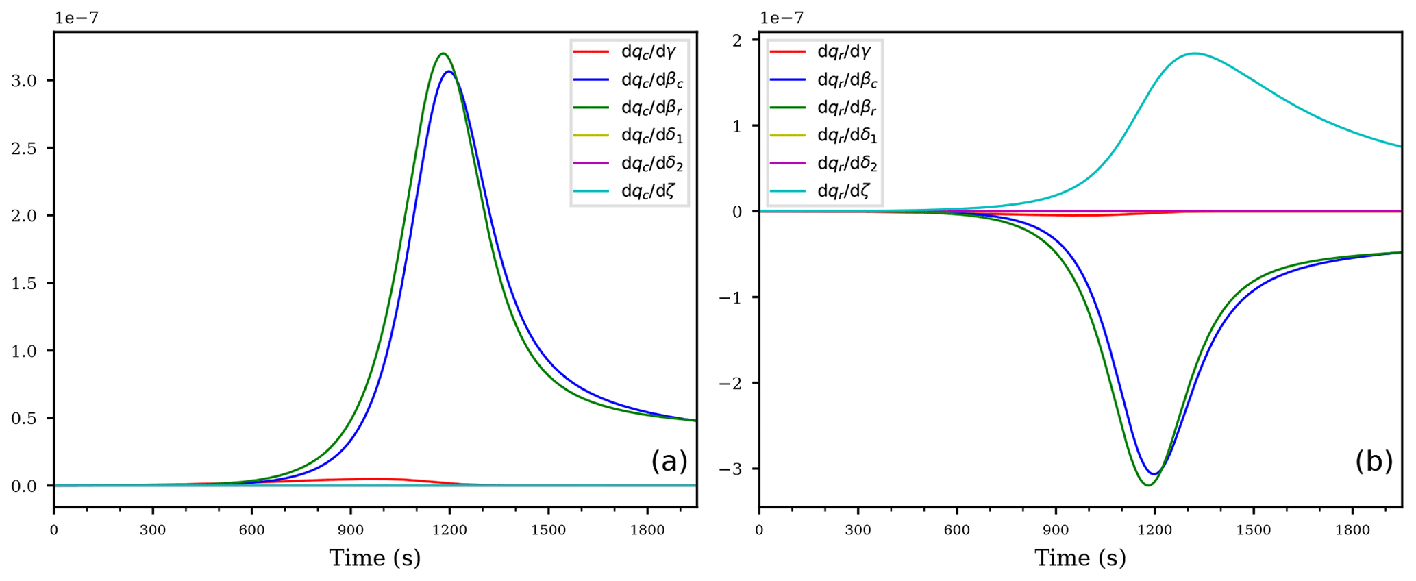
Figure 3As in Fig. 2, but for the derivatives of q_c (a) and q_r (b) with respect to the exponents.

Download

Figure 3 shows the derivatives of the mixing ratios q_c, q_r with respect to the exponents. For both mixing ratios, obviously the exponents β_c, β_r from the accretion process are most sensitive (blue and green curves).

Note that the sign of the curves is counter intuitive, because, e.g., positive values of the blue and green curves imply slower accretion after increasing the values of those exponents by a small amount. This behavior is easily explained with the values of both mixing ratios being smaller than unity: increasing the exponent in the expression $a_{\mathrm{2}}{q}_{\mathrm{c}}^{{\mathit{\beta }}_{\mathrm{c}}}{q}_{\mathrm{r}}^{{\mathit{\beta }}_{\mathrm{r}}}$ with $\mathrm{0}\le q_{\mathrm{c}},q_{\mathrm{r}}<\mathrm{1}$ leads to decreased values of the expression $a_{\mathrm{2}}{q}_{\mathrm{c}}^{{\mathit{\beta }}_{\mathrm{c}}}{q}_{\mathrm{r}}^{{\mathit{\beta }}_{\mathrm{r}}}$ and consequently to a slower accretion process. It is important to keep such a behavior in mind in interpreting the derivatives.

The second most sensitive exponent for the rain mixing ratio is given by exponent ζ from the sedimentation process, but only after enough rain drop mass has formed after about 1000 s. The magnitude of the derivatives with respect to ζ and the accretion exponents β_c, β_r are comparable and of opposite sign. Therefore, the influence of increasing these exponents simultaneously may cancel out.

Observe that the derivatives of both mixing ratios with respect to the exponents δ₁, δ₂ in Fig. 3 are exactly zero, again resembling the in-activeness of the evaporation term in Eq. (12c) within the supersaturated cloud parcel.

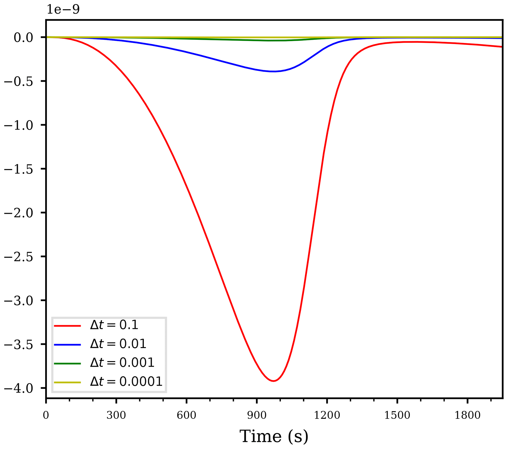
Figure 4Temporal evolution of the derivative $\frac{\partial q_{\mathrm{c}}}{\partial a_{\mathrm{1}}}$ using the time steps $\mathrm{\Delta }t\in \mathit{\{}\mathrm{0.1},\mathrm{0.01},\mathrm{0.001},\mathrm{0.0001}\mathrm{s}\mathit{\}}$ for the computation of the same case as in Fig. 2.

Download

As indicated, AD computes the derivatives of the implemented code, which in our case involves a numerical method, rather than derivatives of the (unknown) continuous solution of the governing differential equation. This distinction is important for the interpretation of the computed sensitivities and we are now going to discuss the subtleties connected with them.

First of all, we outline the fact that since the numerical discretization of the governing differential equation depends on the time step Δt, the magnitude of all computed derivatives also depend on the time step. Figure 4 illustrates this fact by showing the derivative $\frac{\partial q_{\mathrm{c}}}{\partial a_{\mathrm{1}}}$ of the cloud droplet mass on the parameter a₁ for autoconversion for several time steps. In this figure, the dependency on Δt becomes obvious, however, the shape of the curve does actually not change. Rescaling the curves in Fig. 4 by multiplying the values of the blue curve by $\frac{\mathrm{0.1}}{\mathrm{0.01}}=\mathrm{10}$, the values of the green curve by $\frac{\mathrm{0.1}}{\mathrm{0.001}}=\mathrm{100}$, and the values of the yellow curve by $\frac{\mathrm{0.1}}{\mathrm{0.0001}}=\mathrm{1000}$, all rescaled curves coincide with the red curve (not shown), representing the derivative computed with time step Δt=0.1. Although this scaling with the time step is quite intuitive due to the fact that if the time step is larger, the simulation is done for a larger time interval and the sensitivities are expected to increase, one should be aware of this scaling when trying to interpret the magnitudes of the derivatives.

A second issue regarding the meaning of the computed sensitivities is addressed in Bischof and Eberhard (1999). There are two possibilities of computing sensitivities:

1. apply AD on the implemented code, which numerically approximates the unknown solution of the governing differential equation, or

2. derive an analytical differential equation (called the sensitivity or variational equation as an analogue of the forward AD mode or the adjoint equation as an analogue of the reverse AD mode), describing how the sensitivities evolve with time (see, e.g., Sandu et al., 2003, or Walther, 2007, for details). In this approach, AD may enter the computation of the derivatives of the right-hand side of the governing equation.

The essential difference between the possibilities is that the first approach explicitly includes the numerical method in the computation of the sensitivities, while the second approach excludes any numerical method in the first place and instead creates an analytical differential equation, e.g., the sensitivity equation, for the description of the sensitivities and only in a second step approximates the exact solution of this equation using a numerical method.

In our study we choose the first option and include the numerical method in the differentiation, since this seems more appropriate if one is interested in how the sensitivities propagate through a given, already implemented, numerical model. We use a one-step numerical method with constant time step Δt to approximate the ordinary differential equation, hence the numerical solution y^new at the new time level is connected to the old solution y^old at the old time level by $y^{\mathrm{new}}=y^{\mathrm{old}}+\mathrm{\Delta }t\cdot \mathrm{\Phi }(y^{\mathrm{old}},\mathit{\eta },\mathrm{\Delta }t)$, where η represents the parameter vector as in Eq. (17) and Φ is the numerical method. Moreover, we compute the derivatives at each time step separately, i.e., the approximation y^old is considered as independent of the parameters at the current time level, hence $\frac{\partial y^{\mathrm{old}}}{\partial \mathit{\eta }}=\mathrm{0}$. Consequently, in our case the AD methodology factually computes the derivative

$$\begin{array}{}\text{(19)}& \begin{array}{rl}{\displaystyle \frac{\partial y^{\mathrm{new}}}{\partial \mathit{\eta }}}& ={\displaystyle \frac{\partial y^{\mathrm{old}}}{\partial \mathit{\eta }}}+\mathrm{\Delta }t\cdot {\displaystyle \frac{\partial }{\partial \mathit{\eta }}}\left[\mathrm{\Phi }(y^{\mathrm{old}},\mathit{\eta },\mathrm{\Delta }t)\right]\\ & ={\displaystyle \frac{\partial y^{\mathrm{old}}}{\partial \mathit{\eta }}}+\mathrm{\Delta }t\cdot \left[{\displaystyle \frac{\partial \mathrm{\Phi }}{\partial y}}(y^{\mathrm{old}},\mathit{\eta },\mathrm{\Delta }t){\displaystyle \frac{\partial y^{\mathrm{old}}}{\partial \mathit{\eta }}}\right.\\ & \left.+{\displaystyle \frac{\partial \mathrm{\Phi }}{\partial \mathit{\eta }}}(y^{\mathrm{old}},\mathit{\eta },\mathrm{\Delta }t)+{\displaystyle \frac{\partial \mathrm{\Phi }}{\partial \mathrm{\Delta }t}}(y^{\mathrm{old}},\mathit{\eta },\mathrm{\Delta }t){\displaystyle \frac{\partial \mathrm{\Delta }t}{\partial \mathit{\eta }}}\right]\\ & =\mathrm{\Delta }t\cdot {\displaystyle \frac{\partial \mathrm{\Phi }}{\partial \mathit{\eta }}}(y^{\mathrm{old}},\mathit{\eta },\mathrm{\Delta }t),\end{array}\end{array}$$

showing once again the observed dependency of the computed sensitivities on the time step. In addition, Eq. (19) shows explicitly that the numerical method Φ is included in the differentiation, and thus the computed sensitivities depend on the numerical method. Note that we employed a constant time step that, according to the results in Bischof and Eberhard (1999), ensures that the computed sensitivities are indeed approximations of the sensitivities of the unknown, exact solution. If we had used a numerical method with adaptive time-stepping, this would not necessarily be true, since in this case the current time step depends on the solution which in turn depends on the parameters η, implying $\frac{\partial \mathrm{\Delta }t}{\partial \mathit{\eta }}\ne \mathrm{0}$ in general. Again, if one is interested in an approximate computation of the sensitivities of the exact solution, a correction is needed for this non-zero contribution of $\frac{\partial \mathrm{\Delta }t}{\partial \mathit{\eta }}\ne \mathrm{0}$; see Bischof and Eberhard (1999). However, if one is interested in the sensitivities of the implemented code, no correction is needed.

Finally, it is not obvious that the computed sensitivities, which depend on the time step, converge to the sensitivities of the exact but unknown solution in the limit Δt→0. In our case, since we rely on an explicit Runge–Kutta method of order 4, the desired convergence is established in Walther (2007). An extension to a more general Runge–Kutta method for the adjoint equation is presented in Sandu (2006).

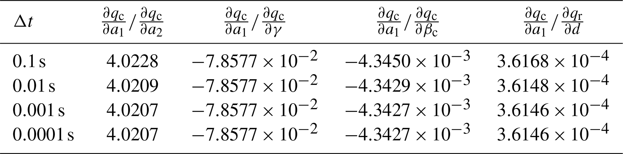
Although the magnitude of the computed derivatives depend on the time step of the numerical method, the relative magnitudes of the individual derivatives are independent of the time step. Table 2 highlights this observation by comparing the ratios of some derivatives of the mixing ratios at t=1000 s, computed with several time steps Δt. The ratios of the derivatives shown in Table 2 are indeed approximately constant (except for the effects of a coarse time resolution), implying that these ratios are indeed independent of the time step. Therefore, the derivative with respect to the most sensitive parameter will show the largest magnitude compared to the derivatives with respect to the other parameters, regardless of the chosen time step of the numerical method involved. This allows the possibility of using the computed derivatives to identify the most sensitive parameters of the cloud scheme.

Table 2Ratios of the derivatives of the mixing ratios with respect to different parameters at t=1000 s, computed for several time steps Δt. All numbers are taken from the computations of the first case of an ascending air parcel with no pre-existing cloud. The numbers are rounded to four digits.

Download Print Version | Download XLSX

4.2 Cloud evaporation in a downdraft

As the second example, we consider a downdraft with velocity $w=-\mathrm{1}\mathrm{m}{\mathrm{s}}^{-\mathrm{1}}$, the initial conditions

$$\begin{array}{}\text{(20)}& \left(q_{\mathrm{c}}\left(\mathrm{0}\right),q_{\mathrm{r}}\left(\mathrm{0}\right)\right)=\left(\mathrm{2}\times {\mathrm{10}}^{-\mathrm{4}}\mathrm{kg}{\mathrm{kg}}^{-\mathrm{1}},{\mathrm{10}}^{-\mathrm{4}}\mathrm{kg}{\mathrm{kg}}^{-\mathrm{1}}\right)\end{array}$$

for the mixing ratios and S(0)=1.01 for the saturation ratio, representing an initial supersaturation of 1 %.

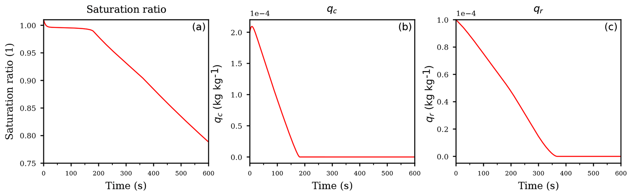
Figure 5Temporal evolution of the saturation ratio S (a), the cloud droplet mixing ratio q_c (b), and the rain drop mixing ratio q_r (c) for the descending air parcel with evaporating cloud.

Download

The temporal evolution of the saturation ratio and the mixing ratios are shown in Fig. 5. The downward vertical motion of the air parcel causes the saturation ratio to decrease due to adiabatic heating. However, until the complete evaporation of the cloud droplets at about 175 s (see Fig. 5b), the release of water vapor of the evaporating cloud droplets counteracts the decrease of the saturation ratio and keeps the air parcel only slightly subsaturated (Fig. 5a). After roughly 175 s, the saturation ratio decreases continuously, resulting in a substantially subsaturated air parcel. Consequently, the available rain drops not only sediment out of the air parcel but also evaporate due to the subsaturation (Fig. 5c). However, the release of water vapor of the evaporating rain drops is seemingly not able to counteract the decrease of the saturation ratio as was the case for the evaporating cloud droplets at the beginning of the simulation, but the precise sensitivities of rain drop evaporation and sedimentation cannot be deduced from the temporal evolution of the mass mixing ratio q_r.

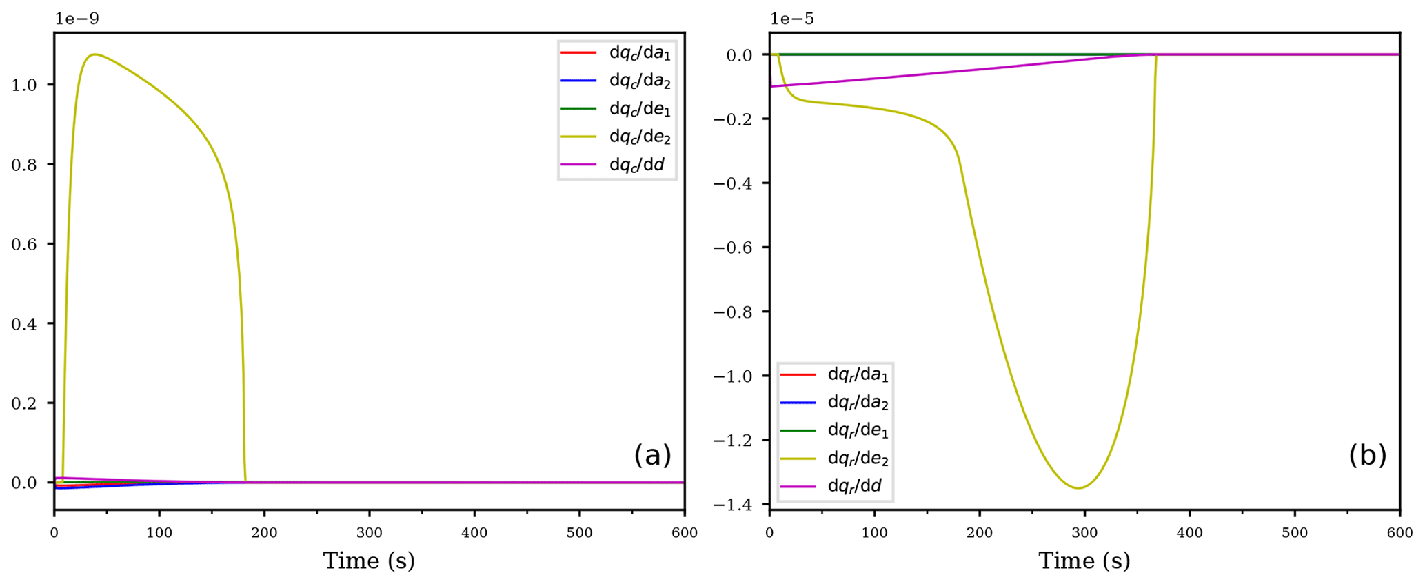
Figure 6Temporal evolution of the derivatives of the cloud droplet mixing ratio q_c (a) and the rain drop mixing ratio q_r (b) with respect to the coefficients for the descending air parcel with evaporating cloud.

Download

The temporal evolutions of the derivatives of the mixing ratios with respect to the coefficients are shown in Fig. 6. Contrary to the first case from Sect. 4.1, the air parcel rapidly becomes subsaturated with S≤1 and the evaporation process in Eq. (12c) is now active, hence no derivative is identically zero. Inspecting Fig. 6, the most sensitive coefficient for both mixing ratios is e₂ (yellow curve), corresponding to the ventilation coefficient within the formulation of the evaporation process of the rain drops; see Eq. (12c). This result may be anticipated regarding the rain drop mass mixing ratio q_r, because the air parcel is subsaturated and the evaporation process directly affects the rain drop mixing ratio. However, we also observe a large sensitivity of the cloud droplet mixing ratio q_c on the same parameter. This feedback is, again, an indirect sensitivity originating from the accretion process: if the rain drop mass decreases faster due to a slight increase of the coefficient e₂, the accretion gets slower and therefore less cloud droplets get collected by the falling rain drops. Consequently, the decrease of cloud droplet mixing ratio is diminished.

Figure 6b also shows that the second most sensitive coefficient for q_r is given by the sedimentation rate coefficient. This observation also answers the question which process is more sensitive to changes in its rate coefficient for the decrease of rain drop mass, seen in Fig. 5b. Due to the larger absolute values of $\frac{\partial q_{\mathrm{r}}}{\partial e_{\mathrm{2}}}$ compared to $\frac{\partial q_{\mathrm{r}}}{\partial d}$ (yellow and purple curves in Fig. 6b), a slight change in the evaporation rate coefficient e₂ will result in larger responses than a change in the sedimentation rate.

Although not visible in Fig. 6a, the derivatives with respect to the coefficients $a_{\mathrm{1}},a_{\mathrm{2}},d$ are all of about the same magnitude, while the sensitivity to the second evaporation coefficient e₁ is significantly smaller.

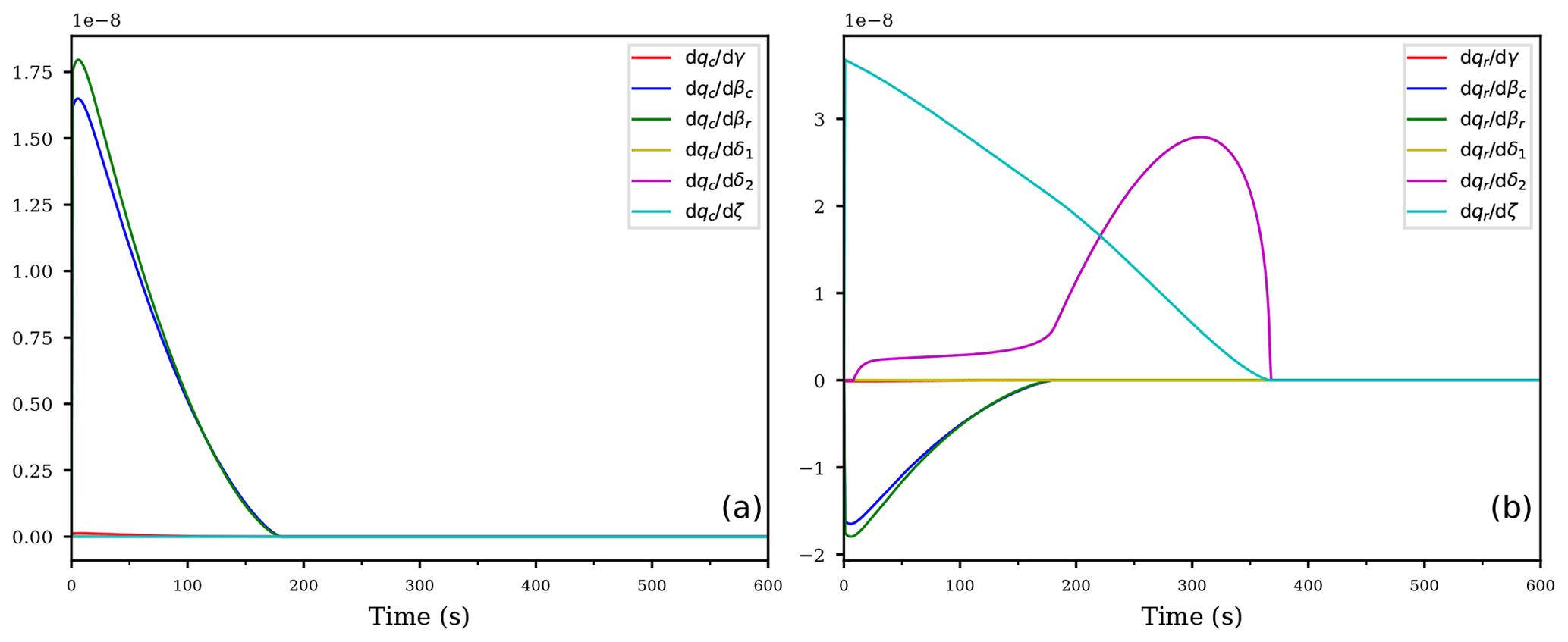
Figure 7As in Fig. 6, but for the derivatives of q_c (a) and q_r (b) with respect to the exponents.

Download

Inspecting Fig. 7, illustrating the derivatives of both mixing ratios to the exponents, the most sensitive exponents for the cloud droplet mixing ratio q_c are again the exponents β_c, β_r corresponding to the accretion process (blue and green curve in Fig. 7a). For the rain drop mixing ratio q_r (Fig. 7b), the most sensitive exponent changes from the sedimentation exponent ζ (cyan curve) at the beginning to exponent δ₂, occurring in the second term $e_{\mathrm{2}}{q}_{\mathrm{r}}^{{\mathit{\delta }}_{\mathrm{2}}}$ of the evaporation term, consistent with the large sensitivity of the corresponding rate coefficient e₂; see the yellow curve in Fig. 6a.

To summarize the second example: the AD methodology pinpoints the second summand $e_{\mathrm{2}}{q}_{\mathrm{r}}^{{\mathit{\delta }}_{\mathrm{2}}}$ of the evaporation term together with the exponents β_c, β_r of the accretion process in introducing the largest sensitivity in the model results. Although one could find the same sensitivities using classical sensitivity studies instead of AD, the AD methodology provides an immediate suggestion on the large sensitivity of the coefficient e₂ for both mixing ratios (see Fig. 6), without having to carry out multiple model runs, where one perturbs each coefficient of the cloud scheme separately, one after the other. Moreover, the sensitivity of the cloud droplet mixing ratio q_c to e₂ is indirect, rendering it difficult to identify this sensitivity directly using the ensemble approach, in particular because the governing Eq. (12a) provides no indication due to the absence of coefficient e₂. Given that even the simple cloud scheme Eq. (12) already contains five rate coefficients, perturbing each coefficient within a separate model run results in a significant total number of runs.

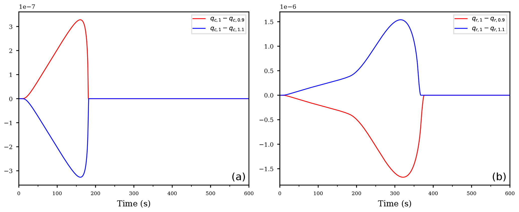
Figure 8Difference between the reference run with unperturbed coefficient e₂, denoted as q_x,1 for $x\in \mathit{\{}c,r\mathit{\}}$ and using the perturbed second evaporation coefficient s⋅e₂ with $s\in \mathit{\{}\mathrm{0.9},\mathrm{1.1}\mathit{\}}$, denoted as q_x,0.9 or q_x,1.1, for the cloud droplet mixing ratio (a) and the rain mixing ratio (b), respectively.

Download

After the identification of the most sensitive parameters using AD, one can carry out further model runs, targeted at the parameters which were identified beforehand. Figure 8 illustrates a possible further analysis step. It shows the difference between an unperturbed run, denoted by q_x,1 with $x\in \mathit{\{}c,r\mathit{\}}$, and two further runs with perturbed rate coefficient s⋅e₂ instead of e₂, where $s\in \mathit{\{}\mathrm{0.9},\mathrm{1.1}\mathit{\}}$ is a scaling parameter. Observe that the signal is consistent with the derivative, computed by AD, in Fig. 6: the derivative $\frac{\partial q_{\mathrm{r}}}{\partial e_{\mathrm{2}}}$ is negative, hence a slight increase of the coefficient should result in a smaller rain mixing ratio q_r and, consequently, the difference of $q_{r,\mathrm{1}}-q_{r,\mathrm{1.1}}$ should be positive. Similarly, the derivative $\frac{\partial q_{\mathrm{c}}}{\partial e_{\mathrm{2}}}$ is positive, and hence a slight increase of the coefficient should result in negative values for the difference $q_{c,\mathrm{1}}-q_{c,\mathrm{1.1}}$. Figure 8 shows exactly these tendencies (blue curves). The red curves show the resulting differences using the scaling parameter s=0.9; note that the curves are asymmetric to each other.

The code for the cloud model together with all scripts needed to reproduce the results in this study are available at https://doi.org/10.5281/zenodo.3461483 (Baumgartner, 2019). The algorithmic differentiation tool CoDiPack may be found online at https://github.com/scicompkl/codipack (last access: 6 December 2019) and the version 1.8.1, which is used in this study, is available at https://doi.org/10.5281/zenodo.3460682 (Sagebaum et al., 2019).

MB developed the cloud model code and carried out the numerical experiments under the supervision of AB and PS. MS developed the algorithmic differentiation tool CoDiPack under the supervision of NRG. MB and MS prepared the manuscript with reviews from NRG, AB, and PS.

The authors declare that they have no conflict of interest.

This research has been supported by the Deutsche Forschungsgemeinschaft (grant nos. 320898076 and 257899354).

This paper was edited by David Topping and reviewed by two anonymous referees.