the Creative Commons Attribution 4.0 License.
the Creative Commons Attribution 4.0 License.
 | 20 Feb 2019
Using observed river flow data to improve the hydrological functioning of the JULES land surface model (vn4.3) used for regional coupled modelling in Great Britain (UKC2)
Alberto Martínez-de la Torre
Eleanor M. Blyth
Graham P. Weedon
Land surface models (LSMs) represent terrestrial hydrology in weather and climate modelling operational systems and research studies. We aim to improve hydrological performance in the Joint UK Land Environment Simulator (JULES) LSM that is used for distributed hydrological modelling within the new land–atmosphere–ocean coupled prediction system UKC2 (UK regional Coupled environmental prediction system 2). Using river flow observations from gauge stations, we study the capability of JULES to simulate river flow at 1 km2 spatial resolution within 13 catchments in Great Britain that exhibit a variety of climatic and topographic characteristics. Tests designed to identify where the model results are sensitive to the scheme and parameters chosen for runoff production indicate that different catchments require different parameters and even different runoff schemes for optimal results. We introduce a new parameterisation of topographic variation that produces the best daily river flow results (in terms of Nash–Sutcliffe efficiency and mean bias) for all 13 catchments. The new parameterisation introduces a dependency on terrain slope, constraining surface runoff production to wet soil conditions over flatter regions, whereas over steeper regions the model produces surface runoff for every rainfall event regardless of the soil wetness state. This new parameterisation improves the model performance across Great Britain. As an example, in the Thames catchment, which has extensive areas of flat terrain, the Nash–Sutcliffe efficiency exceeds 0.8 using the new parameterisation. We use cross-spectral analysis to evaluate the amplitude and phase of the modelled versus observed river flows over timescales of 2 days to 10 years. This demonstrates that the model performance is modified by changing the parameterisation by different amounts over annual, weekly-to-monthly and multi-day timescales in different catchments, providing insights into model deficiencies on particular timescales, but it reinforces the newly developed parameterisation.
- Article
(4602 KB) - Full-text XML
- BibTeX
- EndNote


The land surface provides a two-way link between terrestrial hydrology and meteorology. Improving the representation of runoff generation in models of the land surface which are coupled to the atmosphere and oceans could potentially improve meteorological forecasts as well as hydrological predictions. For the UK, a fully coupled (land, atmosphere, ocean) environmental prediction system is being built at 1.5 km2 spatial resolution (UKC2; Lewis et al., 2018). The land surface component of this coupled system is the Joint UK Land Environment Simulator (JULES) model. In this paper, we focus on the runoff generation process. Improved assessments of runoff to the sea surrounding the UK will affect sea surface salinity and therefore influence meteorological forecasts in the UK. Furthermore, the representation of runoff generation in a land surface model will affect coupled system predictions in terms of atmospheric moisture availability, because it modifies other processes of the water cycle, such as evapotranspiration fluxes and surface energy partition.
Different stages of the development of the JULES capability for this process have been published (Best et al., 2011; Blyth, 2002; Clark and Gedney, 2008), and analyses of runoff outputs has been carried out at the site level (Blyth, 2002; Blyth et al., 2011; Weedon et al., 2015) for a set of Rhône subcatchments treated as single grid cells (Clark and Gedney, 2008) and on the global scale with JULES simulations at 0.5∘ or 1∘ (Blyth et al., 2011; Gudmundsson et al., 2012; Papadimitriou et al., 2016, 2017). However, a regional-scale analysis of the process at ∼1 km2 spatial resolution was needed in order to implement an appropriate JULES hydrological parameterisation for the coupled system within UKC2.
Runoff in land surface models (LSMs) is typically represented as the sum of surface runoff and baseflow. Most current LSMs (JULES included) simulate surface runoff as saturation excess, infiltration excess or a combination of these components (Clark et al., 2015; Schellekens et al., 2017). JULES uses the soil hydraulic characteristics to determine the infiltration excess component (Best et al., 2011) and a parameterisation of the saturated fraction of the soil representing the subgrid variability of soil moisture to determine the saturation excess component (Blyth, 2002; Clark and Gedney, 2008). The subsurface runoff is simulated in many LSMs as the free drainage of water through the bottom of the soil column as represented in the model (e.g. Balsamo et al., 2009; Campoy et al., 2013; Oleson et al., 2010; Walko et al., 2000). JULES provides two options to calculate the baseflow: (a) as subsurface runoff, assuming a simple free drainage approach; or (b) as the lateral subsurface flow within the soil column, adopting a parameterisation in terms of the spatial distribution of topography (Beven and Kirkby, 1979; Clark and Gedney, 2008).
The island of Great Britain represents an ideal platform on which to study the runoff generation in LSMs since it has a range of climatic and topographic characteristics plus a comprehensive set of river flow gauge stations with data stored at the National River Flow Archive (NRFA, UK). The differences in precipitation are high and show a clear west–east and north–south contrast, with yearly means above 10 mm d−1 in western Scotland and below 2 mm d−1 in the south-east of England (CEH-GEAR dataset; Keller et al., 2015; Tanguy et al., 2014). Furthermore, regional precipitation regimes in the island range between 3 and 5 mm d−1 in Scotland and Wales, whereas in the English lowlands (southeast), the mean monthly precipitation varies between 1.5 and 2.5 mm d−1 (Robinson et al., 2017b). In addition to this precipitation variability, topographic differences and varied soil types (e.g. the high permeability of chalky soils in the Thames catchment and other eastern regions; Farrant and Cooper, 2008) result in a wide range of percentage runoff and baseflow index (BFI) responses, reported for the UK by Boorman et al. (1995) in the Hydrology of Soil Types (e.g. BFI = 0.86 for the Avon catchment at Knapp Mill in south-west England and BFI = 0.33 for the Ribble catchment at Samlesbury in north-west England). Hydrological models typically overcome the problem of these regional heterogeneous characteristics as they solve runoff for individual catchments and use parameters calibrated to observed river flow (Bastola et al., 2011; Prudhomme et al., 2010). Nevertheless, there have been significant efforts in the hydrological community to generalise the catchment parameterisation for regional scales (Crooks et al., 2014; Wagener and Wheater, 2006) and to estimate parameters over data-poor or ungauged regions using catchment similarity concepts (Beck et al., 2016; Mizukami et al., 2017). However, a widely used LSM in the research community like JULES requires physically based parameters that produce sensible results on regional and global scales, independently of the region studied (i.e. avoiding local calibration).
In this work we perform, firstly, a sensitivity study of alternative runoff production schemes and parameters to identify the best representation of observed daily river flow at a range of selected catchments in Great Britain. Then, based on those catchment results, we present a novel model development that introduces a topography dependency in the parameter that determines the soil wetness at which a grid cell starts generating saturation excess runoff in relation to the subgrid saturation fraction. The development optimises the generation of daily river flow compared to observations and avoids catchment calibration. Finally, as the ambition of UKC2 is to work towards a coupled prediction system for longer timescales (Lewis et al., 2018), the implications of the new approach are investigated further using cross-spectral analysis to assess the performance against observations over scales ranging from days to multiple years.
2.1 The JULES LSM
The JULES LSM is a widely used community land surface model. It works coupled to the atmosphere in the Unified Model (UM of the UK Met Office), both for operational weather forecasting and for climate applications, as the land surface component of the Hadley Centre family of climate models (HadGEM3 and UKESM1), which are participants in CMIP (https://www.wcrp-climate.org/wgcm-cmip, last access: 13 February 2019). Additionally, JULES can be run uncoupled as a stand-alone tool which is used to assess water resources (e.g. Schellekens et al., 2017; Blyth et al., 2019) and to study land–atmosphere interactions and impacts (Betts, 2007; Harrison et al., 2008; Van den Hoof et al., 2013). Details of the structure and processes represented in JULES are described by Best et al. (2011; energy and water fluxes) and Clark et al. (2011; carbon fluxes and vegetation dynamics).
JULES divides the land into grid boxes and resolves subdaily water and energy fluxes at the land surface and through vertical soil layers (typically 4 layers of 0.1, 0.25, 0.65 and 2.0 m thickness, down to 3.0 m). A detailed description of the model hydrological methods is given in Best et al. (2011), and a thorough description of the hydrological processes in JULES from the water reaching the land surface as precipitation is given in Blyth et al. (2019). Here, we focus on the runoff production process and its parameter variability.
Runoff generation and river routing schemes in JULES
From the precipitated water that arrives at the surface after vegetation interception at each model time step, JULES first determines the infiltration excess component of surface runoff from the soil hydraulic characteristics (Best et al., 2011; Blyth et al., 2019). Then, for saturation excess surface and subsurface runoff, two scheme options representing subgrid variability can be used. These approaches are thoroughly described by Clark and Gedney (2008); one based on the probability distributed model (PDM; Moore, 1985, 2007, first included in JULES by Blyth, 2002) and the other one based on TOPMODEL (Beven and Kirkby, 1979).
The PDM approach in JULES calculates the fraction of each model grid box that is saturated as water infiltrates into the soil and the soil storage is filled. This fraction is given by the following:
where S is the areal fraction of grid-box soil water storage, S0 is the minimum storage at and below which there is no surface saturation (note that fsat=0 for S≤S0), Smax is the maximum grid-box storage: Smax=θsatzpdm, where θsat is the volumetric soil water content at saturation and zpdm the depth of the soil column considered by the scheme, and b is a shape parameter. Any water from precipitation arriving over the saturated fraction of the grid generates surface runoff. The subsurface runoff, Rb, is obtained as free drainage at the bottom of the soil column, at a rate determined by the soil hydraulic conductivity at the bottom soil layer KN (i.e. Rb=KN; Cox et al., 1999). Therefore, the two parameters that can be used for calibration of PDM within JULES are b and S0.
The TOPMODEL approach also uses a saturated fraction for each model grid box and estimates the saturation excess runoff at the surface as Rs=fsatW0, where W0 is the precipitated water that reaches the topsoil layer. However, within TOPMODEL, fsat is calculated in terms of the grid-box distribution of the topographic index λ that is obtained from subgrid topographic data as the proportion of the grid cell for which the topographic index is higher than a critical value at which the local water table is found at the surface (Best et al., 2011; Gedney and Cox, 2003). The subsurface runoff or baseflow, Rb, is obtained as the lateral subsurface flow:
Λ is the grid-box mean of the topographic index, Ks0 is the saturated conductivity at the surface, α is the anisotropy factor that accounts for differences in the saturation conductivity between the vertical and horizontal directions, f is a decay parameter (also used to implement an exponential decay of the hydraulic conductivity through the soil vertical layers from Ks0 at the surface in the calculation of water vertical transport), and zw is the mean grid-box water table depth calculated as a diagnostic from the grid-box soil moisture profile. Since fsat is constrained by topographic data within TOPMODEL, only f and α parameters can be used for calibration exercises.
Once JULES has calculated the grid-box runoff following either of the approaches described above, the river flow model (RFM; Bell et al., 2007) is used to route surface and subsurface runoff from inland grid cells across the river network and out to sea at each model time step (i.e. subdaily, not at daily steps). RFM is a kinematic wave equation scheme that incorporates scale-dependent parameters and has been recently introduced into JULES (Lewis et al., 2018).
2.2 Selected catchments in Great Britain and experimental set-up
We select 13 catchments in Great Britain (Fig. 1, Table 1). The spatial resolution used for Fig. 1 and all JULES catchment runs for this paper is 1 km × 1 km. These 13 catchments are used in the development of a national hydrological modelling framework (Crooks et al., 2014) and represent a range of soil types, precipitation regimes and geographical locations that characterise the island of Great Britain. We acknowledge the availability of river flow data for a larger number of catchments in the NRFA archive. However, we focus on catchments large enough for the JULES distributed model to integrate hydrological processes on the kilometre scale.
Table 1Information about the selected catchments in Great Britain in Fig. 1. The outlet stations are identified by their National River Flow Archive (NRFA) station number and their name. The annual rainfall from the CEH-GEAR database refers to the studied period (1991–2000). The baseflow index (BFI) data were reported by Boorman et al. (1995).
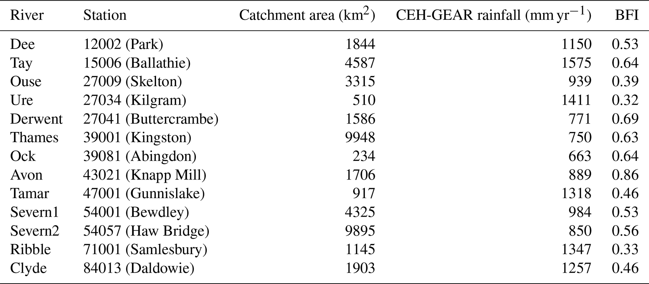
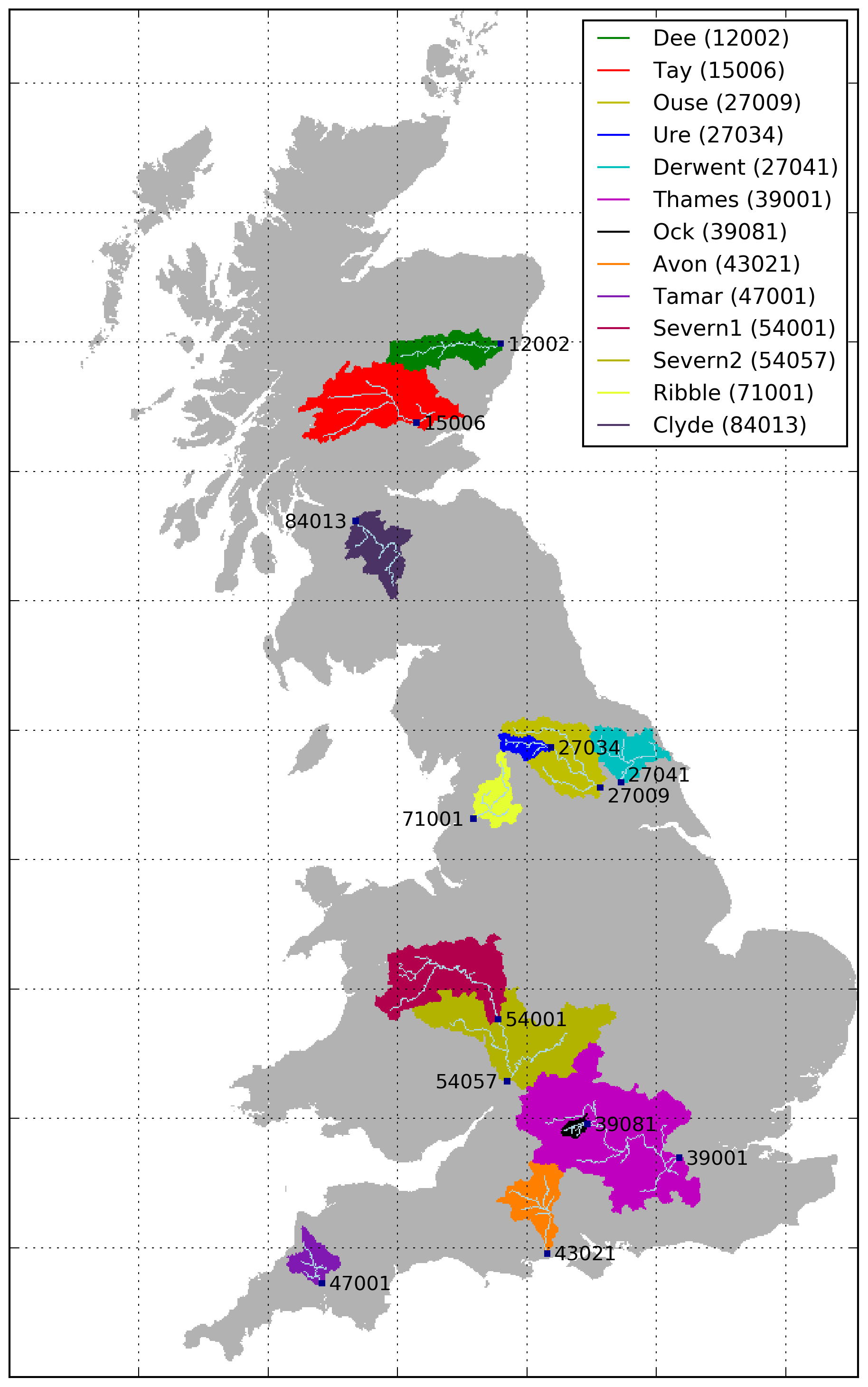
Figure 1Thirteen selected catchments in Great Britain and their main flow pathways. The outlet stations are represented by a dark-blue dot and identified by their National River Flow Archive (NRFA) station number. Note that Ure, Severn1 and Ock are subcatchments within the larger catchments Ouse, Severn2 and Thames, respectively.
2.2.1 Ancillary and driving data
For surface exchanges, JULES divides each land grid cell into a series of tiles that can differ in morphological, physiological and hydrological characteristics according to the land cover. For this work we use the Land Cover Map 2000 (Fuller et al., 2002) produced by CEH (Centre for Ecology and Hydrology, UK), converted to eight different fractional land cover types at the 1 km2 horizontal resolution: broadleaf trees, needleleaf trees, grasses, crops, shrubs, water, bare soil and urban cover. The soil hydraulic characteristics are assumed to be spatially uniform for each grid cell and have been calculated for the model domain from the Harmonized World Soil Database (HWSD; FAO/IIASA/ISRIC/ISS-CAS/JRC, 2012). The topographic index λ has been calculated for Great Britain at 50 m2 resolution from the CEH-IHDTM database (Morris and Flavin, 1990, 1994), following the methodology in Marthews et al. (2015), and then its mean and standard deviation at the 1 km2 model grid are used as input data for the TOPMODEL approach.
The RFM routing scheme uses values of single-flow direction and flow accumulation (number of grid cells flowing to each cell in a river catchment). These river network parameters for the catchments used here were drawn from Davies and Bell (2009), originally calculated from the CEH-IHDTM database (Morris and Flavin, 1990, 1994) following the COTAT algorithm methodology (Paz et al., 2006).
The meteorological driving dataset used to run the model is CHESS-met (Robinson et al., 2017a). This database provides all the required surface variables to run JULES (precipitation, input long-wave and short-wave radiation, air temperature, specific humidity, wind speed and pressure) at 1 km2 spatial resolution for Great Britain and daily time resolution. The precipitation data in CHESS-met are gridded estimates of daily rainfall from gauge stations (CEH-GEAR; Keller et al., 2015; Tanguy et al., 2014), whereas the rest of the variables are interpolated from the observation-based coarser-resolution MORECS dataset (Hough and Jones, 1997; Thompson et al., 1981), taking into account topographic information to disaggregate to the finer scale (Robinson et al., 2017b).
2.2.2 Set of experiments and metrics
A series of test runs is conducted for each catchment in Fig. 1, exploring parameter variability in order to analyse the model performance and find the best hydrological configuration for the simulation of river flow in JULES.
Tests using the PDM scheme include 25 variations of the b shape parameter (b=0.05, 0.1, 0.15, 0.2, 0.25, 0.3, 0.35, 0.4, 0.45, 0.5, 0.55, 0.6, 0.65, 0.7, 0.75, 0.8, 0.85, 0.9, 0.95, 1.0, 1.2, 1.4, 1.6, 1.8, 2.0), controlling the saturation fraction calculation once S0 has been reached. Lower values of b result in lower saturation fraction and therefore less surface runoff during precipitation events. We also add a set of tests where b is spatially varying as a function of the terrain slope as developed by the Verifications, Impacts and Post-Processing research group in the UK Met Office (unpublished data):
where s is the grid-box terrain slope, smax=21∘, bmin=0 and bmax=0.8. The terrain slope was calculated from the CEH-IHDTM database (Morris and Flavin, 1990, 1994).
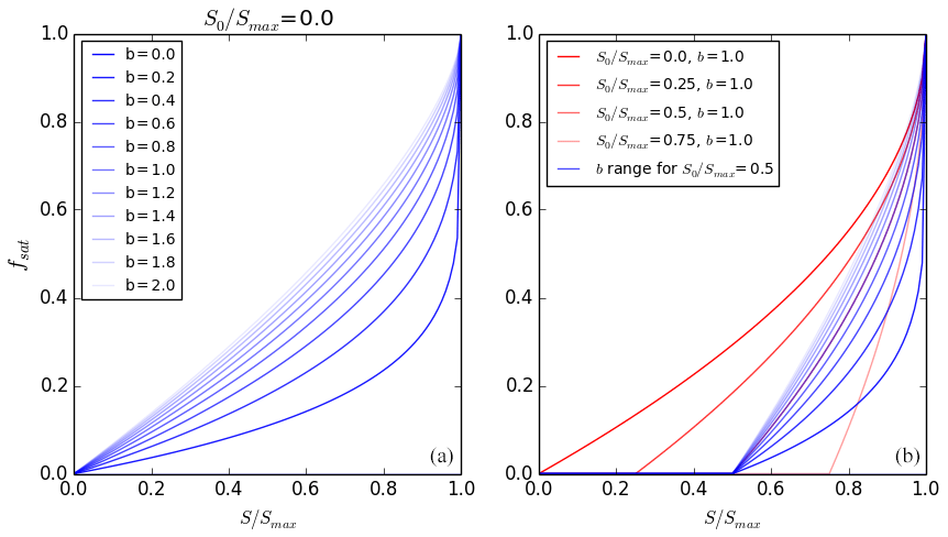
Figure 2(a) Variability of the soil moisture saturation fraction introduced by the b parameter in the PDM scheme, for S0/Smax=0.0. (b) Variability of the soil moisture saturation fraction introduced by the S0/Smax parameter in the PDM scheme, for b=1.0 (red lines) and variability introduced by the b parameter for S0/Smax=0.5 (blue lines).
We choose four possible values for the S0 parameter within the 0–1 range that it can take in the form of fraction of saturation (S0/Smax=0.0, 0.25, 0.5, 0.75), controlling the soil moisture state required to start producing saturation excess surface runoff; i.e. every rainfall event will produce saturation excess runoff when S0/Smax=0.0, even when the soil is dry (reasonable over steep areas where some saturation fraction is always expected), whereas no surface runoff is produced until the saturated area is 25 %, 50 % or 75 % of the grid-cell area in the other three tests (since over flatter terrain a precipitation event might be absorbed entirely by the soil and therefore produce no surface runoff). The combined parameter variability tested in the PDM scheme has a strong effect on the saturated fraction of the soil, with b increasing this fraction at higher values and S0 acting as a constraint on the scheme to start producing saturated fractions and reducing the impact of b variability as its value gets closer to Smax (Fig. 2).
Tests using the TOPMODEL scheme include eight variations of the f decay parameter (f=1.5, 2.0, 2.5, 3.0, 3.5, 4.0, 4.5, 5.0), controlling the decay of hydraulic conductivity with depth and the baseflow production. This range for f is consistent with findings in other JULES studies (Clark and Gedney, 2008; Finney et al., 2012). The anisotropy factor α is related to the soil stratification, and different authors have adopted different values: Chen and Kumar (2001) calibrated it to a value of 2000 for North America, Niu and Yang (2003) used a range of 10–20, Fan et al. (2007) made it dependent on the soil clay content (values between 2 for sand and 48 for clay), and Clark and Gedney (2008) found the value of 100 to best reproduce streamflow with JULES for three Rhône subcatchments. Here, we test four values of the anisotropy factor (α=1, 10, 100, 1000).
Apart from the runoff production at the surface and subsurface, a key configuration for any LSM that simulates the water cycle is the choice of hydraulic model that computes the water movement through the soil profile (Marthews et al., 2014). JULES provides the option of using either the Brooks and Corey (1964) approach (BC) or the Van Genuchten (1980) approach (VG) to represent the hydraulic relationships between soil water content, suction and hydraulic conductivity (Best et al., 2011). BC and VG differ in the way they approach the curves relating the soil water content and the water suction for each soil type; while BC curves tried to best represent available measurements using an exponential fit, VG curves are smoothed to represent an S-shaped relationship suggested by the observations. The differences and potential misrepresentations of both approaches are often found at the dry and wet ends of the curves. The VG asymptotic behaviour can cause non-physical results at the dry end, whereas the BC formulation presents abrupt transition to low water suctions at the wet end, potentially causing model instability (Marthews et al., 2014). For every catchment the PDM and TOPMODEL experiments were run using both the BC and VG approaches, driven by input soil hydraulic properties calculated from the HWSD using the corresponding pedotransfer functions: Cosby et al. (1984) for BC and Wösten et al. (1999) for VG.
Given the range of configuration and parameter combinations, a total of 272 simulations were carried out for each catchment. The simulations cover a total of 10 years (1991–2000) following a 5-year model spin-up (using data from 1986 to 1990). Since the driving CHESS-met dataset is given at daily time steps, a daily disaggregation scheme (Williams and Clark, 2014) allowed JULES to be run at half-hourly time steps. In terms of precipitation, events start at a random time during the day and last for 2 h in the case of convective precipitation and for 6 h in the case of large-scale precipitation.
Although JULES is run at half-hourly time steps, including routing between grid boxes using RFM, the model performance is analysed by comparing the simulations with observed daily river flow data at the catchment outlet stations (Table 1) provided by the NRFA. The Thames at Kingston has a naturalised flow record available (to compensate for flow controls at locks and abstraction), but in all the other catchments the modelled flow is compared directly with the gauged flow.
The Nash–Sutcliffe efficiency (NS; Nash and Sutcliffe, 1970) is used as our baseline metric,
where Qobs,t and Qmod,t are the observed and modelled river flows at a particular time t, T is the total number of observed days, and ‾Qobs is the average observed river flow over the period analysed. NS is widely used in hydrological studies. It measures the accuracy of the model to represent river flow on the given daily timescale and is sensitive to timing differences in peak flows. A value of 1 for NS represents a perfect model, whereas a value of 0 represents no predictive skill (i.e. at NS=0.0 a model performs no better than using the mean river flow). Calculating the average modelled river flow (‾Qmod), we also use the mean bias that indicates the model performance in the long-term balance P−ET (precipitation minus evapotranspiration), calculated as
We acknowledge that river flow simulation model performances using LSMs are influenced by physical processes represented in the model and imposed by the meteorological driving data on multiple timescales. In order to further assess the model performance on timescales longer than a day, which are relevant for the studied catchments, and to complement findings using NS at the daily timescale and mean bias, we use a cross-spectral analysis (Weedon et al., 2015) that provides measurements on how the average amplitude and phase of modelled river flow differ from the observed river flow.
3.1 Soil hydraulics
The main difference between the VG and the BC soil hydraulics formulations is that the VG curve of the soil water suction at soil water contents varies more smoothly close to saturation (Dharssi et al., 2009; Marthews et al., 2014); hence we expect wet soils like those of the catchments in Great Britain used here to be better resolved by the VG approach. Hence we expect the generally wet soils of the catchments in Great Britain used here to be better resolved by the VG approach.
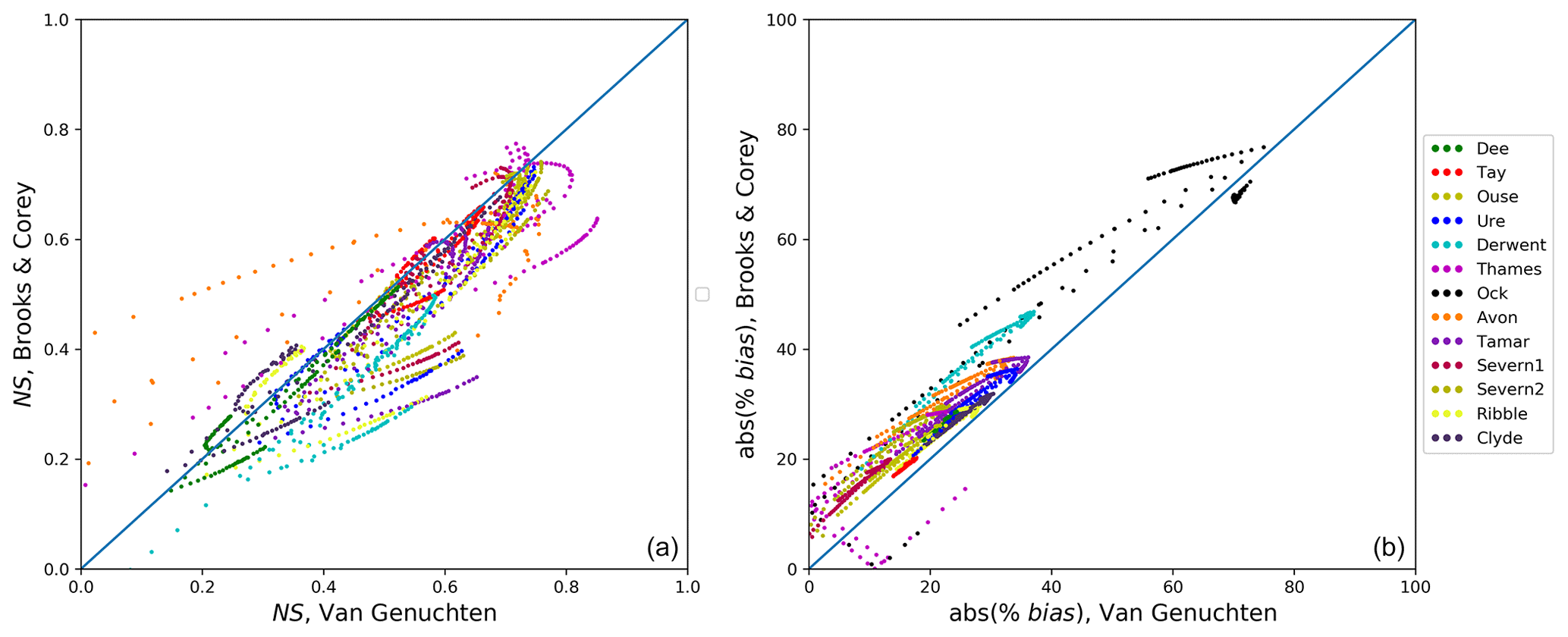
Figure 3River flow performance metrics (NS in a and absolute value of mean bias in b) for all tests conducted and for all 13 catchments (colour code in legend). For any given parameter variability test (single dots), metrics obtained using the BC approach for soil hydraulics formulation are indicated on the y axis and metrics using the VG approach are indicated on the x axis.
NS and mean bias (as its absolute value) metrics from all the catchment tests are shown as scatter plots that compare results obtained using the BC (y axis) and VG (x axis) approaches (Fig. 3). The VG tests perform better in all catchments, as most of the points fall within the VG zone (i.e. below the 1:1 line) in the NS plot (Fig. 3, left), particularly for higher values that indicate better performance. The exception to this result occurs with the Severn1 catchment, where the best NS values of around 0.7 are found using the BC formulation. The BC results show consistently higher absolute bias (i.e. worse performance) than the VG results (Fig. 3, right). Consequently, we will show only results from VG tests in the following plots.
The origin of the pedotransfer functions used to derive soil hydraulic properties further explains the difference in performance shown in Fig. 3 and supports our choice of the VG approach when using JULES for hydrological assessments in Great Britain. For the VG approach the functions were developed from data provided by 20 institutions from 12 European countries, England and Scotland included (Wösten et al., 1999), whereas for the BC approach the original data were taken from 23 localities in the United States (Cosby et al., 1984).
3.2 Sensitivity of runoff generation schemes
The first-order control of variability in runoff generation within JULES is determined by the choice of hydrological scheme: PDM or TOPMODEL. Figure 4 shows the performance metrics obtained for each catchment in all tests.
The mean bias (Fig. 4, right) tends to be negative in most tests, indicating the underestimation of river flow by the model. The TOPMODEL scheme shows low or no range in NS and bias within each catchment, whereas the PDM tests show higher variability within catchments. PDM results range from a high negative bias similar to that of the TOPMODEL results to improved bias (towards zero) across the various tests. The low range in metric values in the TOPMODEL tests was expected, because the f and α parameters tested affect the subsurface runoff production, and therefore the timing of the baseflow discharge, but not directly the surface runoff production through variation of the saturated fraction. As indicated before, the saturated fraction in TOPMODEL is derived from observed topographic characteristics and cannot be calibrated or changed.
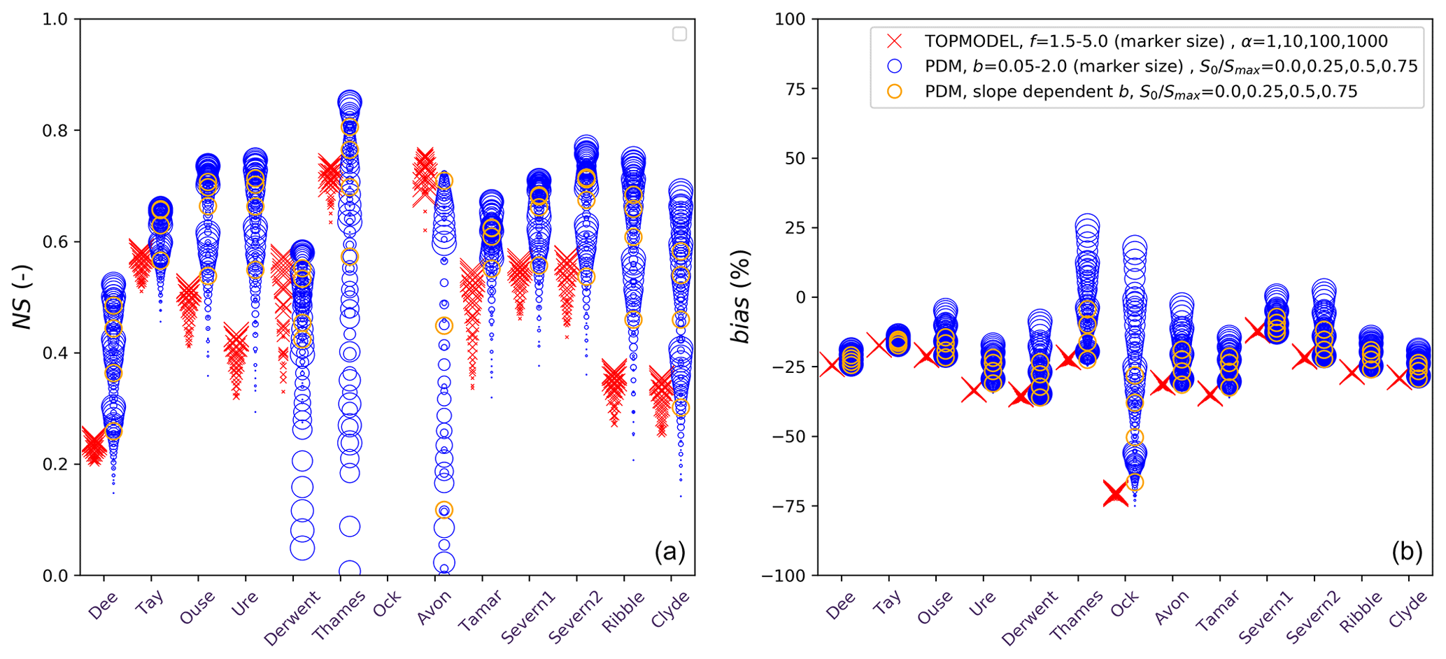
Figure 4River flow performance metrics for catchment tests detailed in Sect. 2.2.2 (red crosses for TOPMODEL tests, blue circles for PDM tests with fixed parameters and orange circles for PDM tests with slope-dependent b). (a) NS efficiency. (b) Mean bias. The x axis represents the 13 selected catchments (Fig. 1). The marker size represents the parameter corresponding to a given tests (and larger crosses for larger f values in the TOPMODEL tests and larger circles for larger b values in the PDM tests). No distinction is shown here indicating the S0/Smax or α parameters. Only results from those tests using the VG approach for soil formulation are shown. Tests at the Ock catchment are not visible since they obtained negative NS.
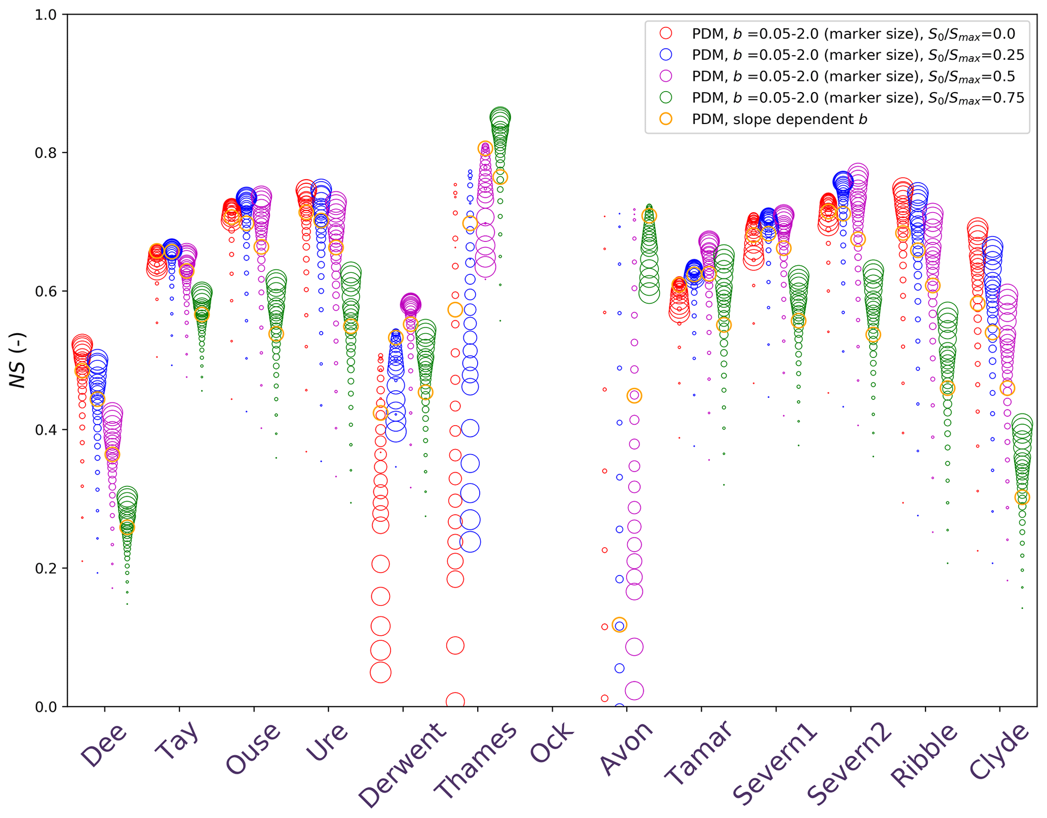
Figure 5River flow NS efficiency performance metric for the PDM catchment tests detailed in Sect. 2.2.2. The x axis represents the 13 selected catchments (Fig. 1). The marker colour represents the S0/Smax value (red, blue, purple and green for values of 0.0, 0.25, 0.50 and 0.75, respectively) and the marker size represents the b parameter (larger circles for larger b values). The slope-dependent b tests are represented by orange markers. Only results from those tests using the VG approach for soil formulation are shown. Tests at the Ock catchment are not visible since they obtained negative NS.
The NS metric (Fig. 4, left) shows a larger range according to the parameters used in the PDM tests and, overall, reaches higher values (closer to 1), indicating the potential for a better performance. Only for the baseflow-dominated catchments (BFI ≥ 0.6; Tay, Derwent, Thames and Avon), do the TOPMODEL results approach the better PDM NS results. This might be because baseflow in TOPMODEL is more sensitive to the parameters that are tested. The TOPMODEL river flow production gets poor NS metric values (below 0.4) on other catchments towards the north with higher total precipitation and lower BFI (i.e. for the Dee, Ribble and Clyde).
The constraint introduced by the S0 parameter in the PDM scheme seen in Fig. 2 results in an added degree of variability to the PDM tests. The bias becomes more negative as S0 increases, indicating less river flow at the catchment outlets and a poorer representation of the P−E balance. However, at baseflow-dominated catchments like the Thames, Derwent, Avon or the Severn2, the NS metric clearly improves for higher S0 (Fig. 5). Considering the b parameter variability, there is a general overall improvement of performance for higher values of b (increasing NS as the marker size increases in Fig. 5). This is not clear for all catchments: the two Severn catchments and the northern Tay catchment reach the best performance (NS) at b values of around 0.5–0.6 for the S0=0 tests (red markers). Over other catchments with discharge heavily influenced by baseflow (Thames, Avon and Derwent), the lowest values of b produce the higher NS metrics when S0 is low. Conversely, high values of b produce the best NS metrics for these catchments as S0 increases. The slope-dependent b parameter tests produce good predictive skill in some instances, but are consistently outperformed by other tests with fixed parameters.
3.3 Optimising the PDM parameters
The results in Sect. 3.2 suggested that the PDM approach can produce better results than the TOPMODEL approach in terms of river flow simulation for the selected catchments. However, the best possible PDM parameters vary for each catchment. In this section, we describe how we developed a universal method for optimising parameter estimation based on topographic data.
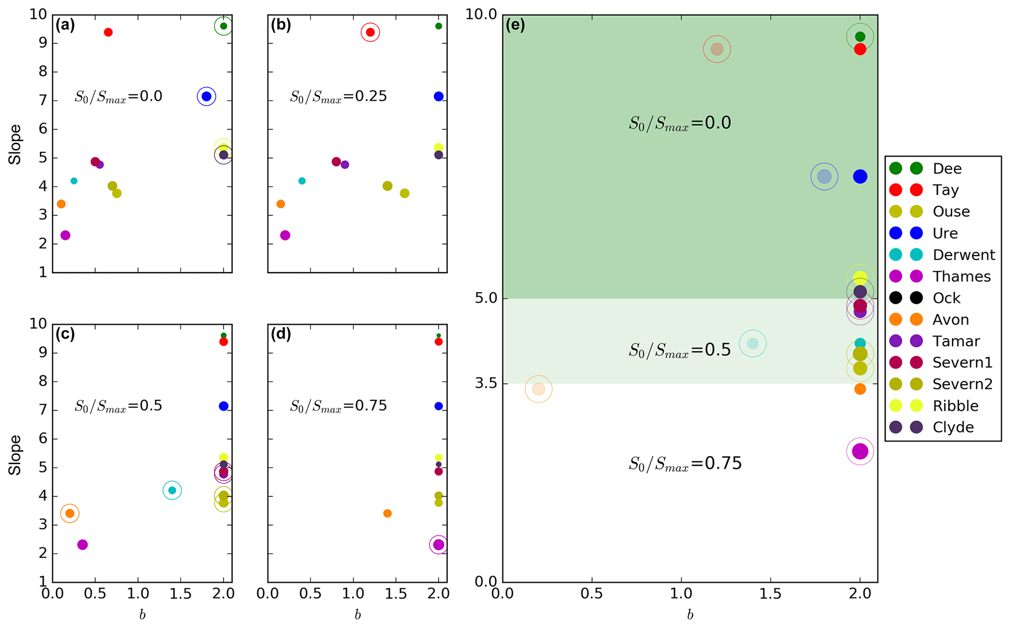
Figure 6(a–d) Representation of the b parameter value (x axis) of catchment tests that obtained a better NS metric for a given value of S0∕Smax (stated inside each plot) against the mean catchment slope on the y axis. The marker size represents the NS values (larger circles for higher NS values). Tests highlighted with an outer circle indicate the best performance of all tests for a given catchment (so the panel where they are indicates S0∕Smax and the x value indicates b). Tests where the mean bias is higher than 30 % are not considered due to a poor performance. (e) Best PDM-parameter tests selected for each catchment following the criterion mcs of fixed b=2 and slope-dependent value of S0∕Smax are as follows: 0.0 for mean catchment slopes higher than 5.0∘ (green background), 0.5 for mean catchment slopes between 3.5 and 5.0∘ (light green background), and 0.75 for mean catchment slopes lower than 3.5∘ (white background). For those catchment in which mcs does not select the test of the best NS metric (Tay, Ure, Derwent, Avon), the best-performing tests are also represented with a degree of transparency.
In Fig. 6, we relate the best-performing PDM parameters to the physical parameter that shows the dominant correlation with the performance results: the mean terrain slope of the particular catchments. The terrain slope was calculated depending on elevations in a 3×3 grid-cell neighbourhood (Horn, 1981) using the elevation data at 50 m2 resolution from the CEH-IHDTM database (Morris and Flavin, 1990, 1994) and then calculating the mean angle at the working resolution of 1 km2. Plots on the left in Fig. 6a–d illustrate how the mean catchment slope can help determine the optimum PDM parameters: (1) the Thames is the flattest catchment (mean slope of 2.3∘) and the only one where the highest S0 produces the best result, (2) there are a series of catchments with mean slope in the range 3.5–5∘, where S0/Smax=0.5 produces the best performance, and (3) the catchments with mean slope above 5∘ produce the best results with S0/Smax=0.0.
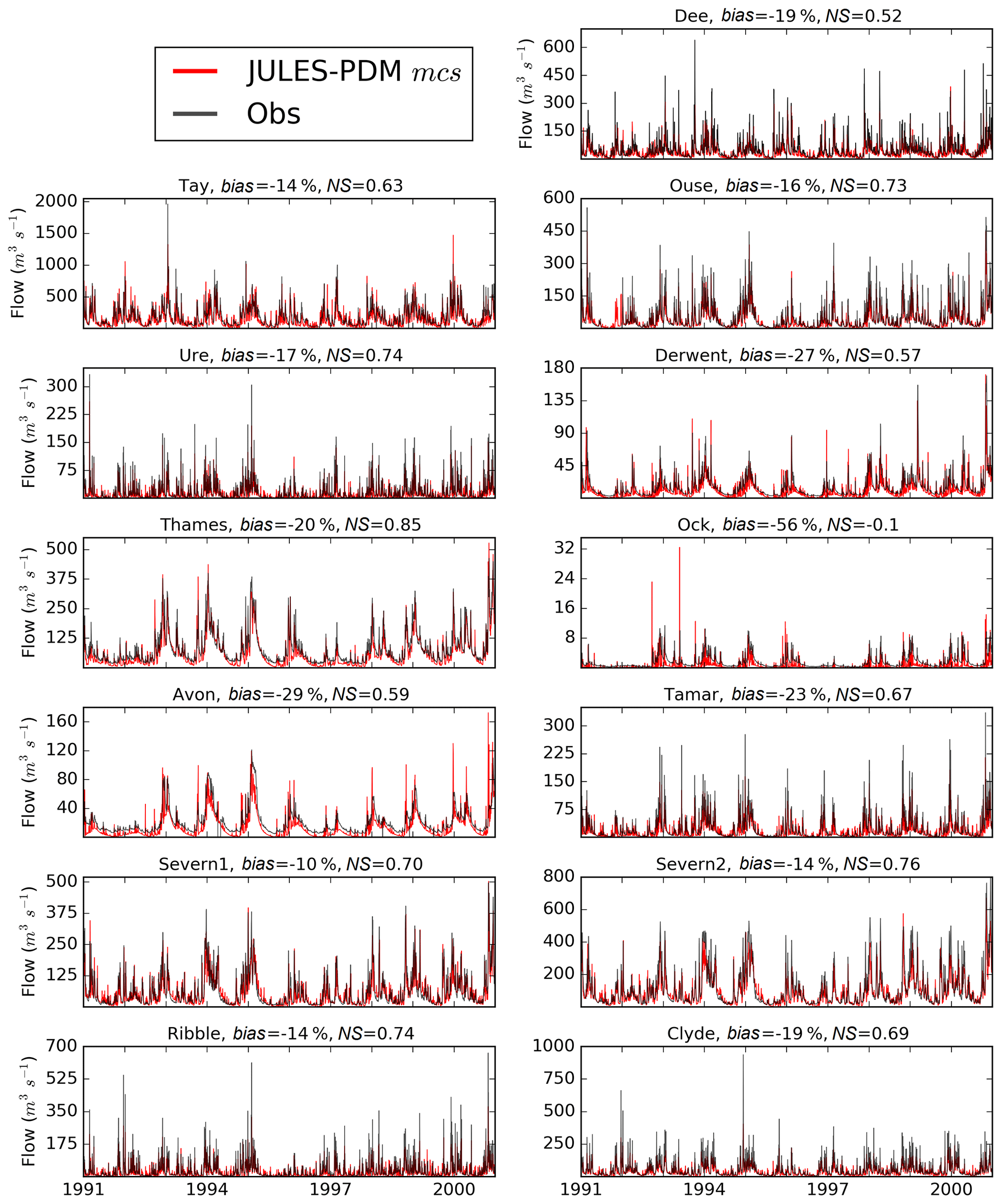
Figure 7Daily river flow (1991–2000) for the 13 catchments studied (Fig. 1). Observations at the NRFA gauge station (Table 1) in black and simulations at the outlet grid by JULES using the criterion mcs in red. On top of each plot the name of the catchment and the performance metrics (mean bias and the NS) are given.
Focusing on the b parameter value represented on the x axis of Fig. 6, the best performance for each catchment (markers highlighted with an outer circle) is consistently found towards the high end of the parameter range, with the exception of the Tay, Derwent and Avon catchments. Hence, we propose a new criterion for simulating river flow for catchments in Great Britain (Fig. 6e) based on the mean catchment slope (mcs hereafter), with a fixed b=2.0 and a simple choice of S0/Smax=0.75 for catchment slopes below 3.5∘, S0/Smax=0.5 for catchment slopes between 3.5 and 5∘, and S0/Smax=0.0 for catchment slopes above 5∘. When applying this new mcs criterion (daily river flow time series and evaluation metrics shown in Fig. 7), the JULES performance in most of the 13 catchments is as good as when using the PDM parameters that produce the best performance (shown by highlighted markers in Fig. 6e). A clear exception is the Avon catchment, where the NS metric is reduced from 0.68 to 0.60 when changing from the best found performance to mcs. The other catchments where mcs does not exactly match the best-performing tests are the Tay, Ure and Derwent. On the other hand, in these catchments, NS does not change when switching to use of the mcs criterion (Ure, NS = 0.74; Derwent, NS = 0.57) or is only slightly reduced (Tay, from 0.66 to 0.63).
By applying the mcs criterion we are able to introduce catchment variability in the JULES performance related to different topography characteristics, which reaches high NS values in flat catchments, such as the Thames, with baseflow-dominated runoff, and in steeper catchments, such as the Ouse and Ribble, with fast surface runoff production during rainfall events and low BFI.
3.4 Applying the new criterion mcs at the grid resolution
A key driver for this work in the context of developing a UK regional coupled environmental prediction system (UKC2; Lewis et al., 2018) is to develop the best possible representation of the hydrology in JULES for the whole Great Britain domain and at a resolution close to the coupled model resolution (approximately 1.5 km2 at midlatitudes). It is therefore necessary to be able to apply the new criterion on 1 km2 grid cells rather than in particular catchments (note that mcs is based on catchment-wide PDM parameters for each test). To develop spatially varying parameter sets, a S0/Smax parameter dependency on terrain slope at the model grid-cell resolution is considered. We adopt a simple approach using a linear dependency of S0/Smax on slope for values below a given threshold, representing the PDM parameters in the mcs criterion presented in Sect. 3.3 at the model grid-cell resolution, as follows:
where s is the grid-cell slope and smax is the maximum slope that results in S0/Smax higher than zero (smax=6∘ obtained the best results in the case of JULES stand-alone simulations using the 1 km2 slope data described in Sect. 3.3). Effectively, the inclusion of this slope dependency limits the saturation excess runoff production within flatter regions in wet situations, and it enhances runoff production within steeper regions due to a high b parameter with no limitation due to soil water content.
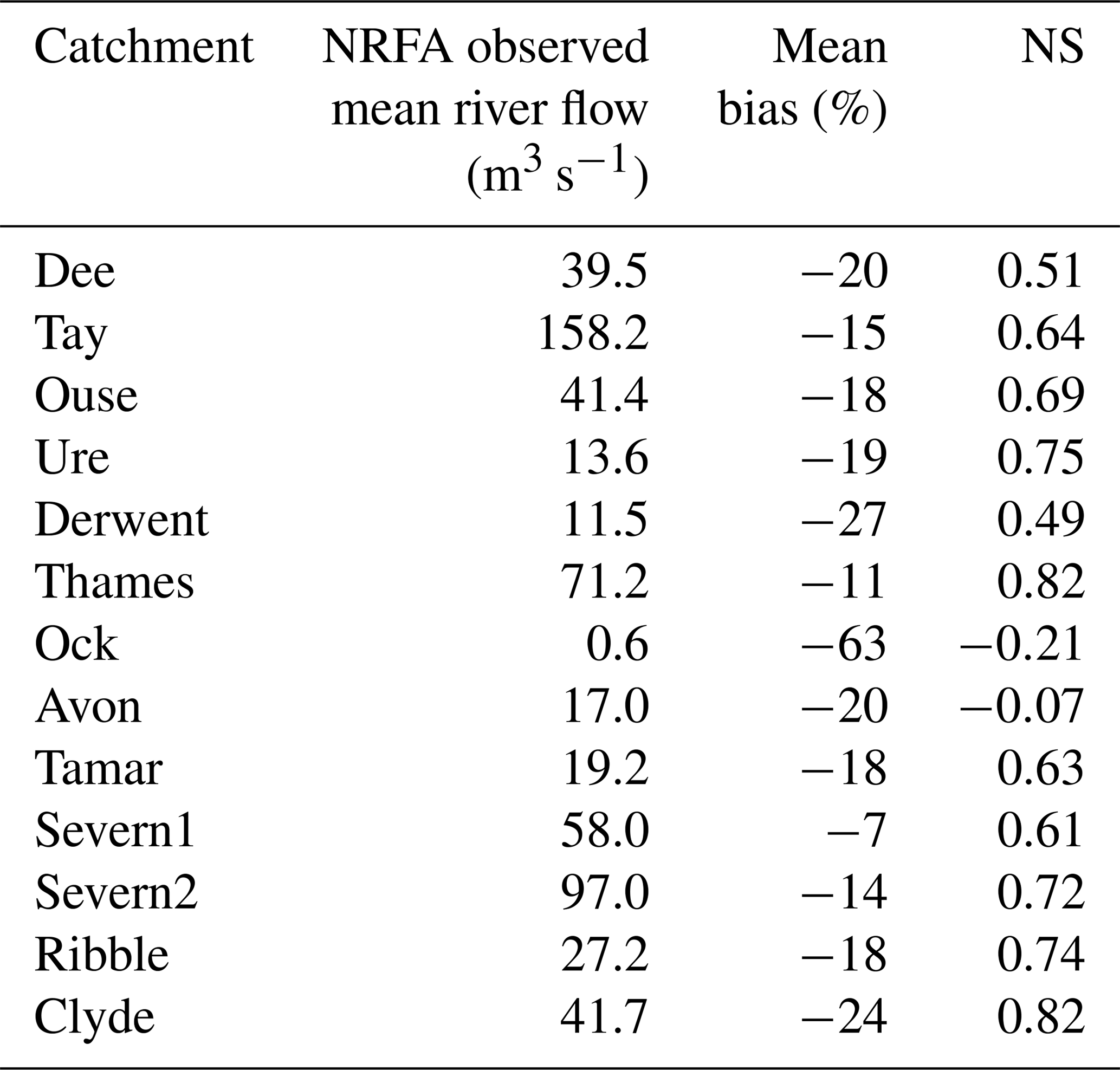
We introduce this linear function for a grid-cell slope dependency in the S0/Smax parameter in the JULES model and integrate a new simulation for each catchment, obtaining the river flow performance metrics reported in Table 2. We stress at this point that the results do not have predictive skill at the Avon and Ock catchments. The Avon is the main outlier in this study due to an unsaturated chalk zone which has known fast flow in the subsurface and might require a different soil hydrology modelling altogether (Rahman and Rosolem, 2017; Blyth et al., 2019). The Ock is the smallest catchment of the selection (234 km2), located upstream within the Thames basin (mean observed river flow of 0.6 m3 s−1), and its results indicate that for upstream small catchments the slope dependency alone does not necessarily solve the parameterisation problem (the Ock does not possess as low a mean slope as the Thames as a whole; see Fig. 6). However, for the whole Thames catchment our new parameterisation achieves the best result of all selected catchments (NS=0.82).
Table 2Mean observed river flow at the 13 selected catchments in Great Britain and performance metrics for JULES using the PDM parameters detailed in Sect. 3.4 (fixed b=20 and grid-cell slope-dependent S0/Smax).
3.5 Performance comparisons using a hydrological model of Great Britain as a benchmark
We show the performance metrics for daily river flow simulations using grid-cell slope dependency for the parameter S0/Smax over the 13 catchments studied (Fig. 8) and illustrate the daily river flow time series for the three larger catchments over 2 years (Fig. 9). We define three performance categories in Fig. 8 following Crooks et al. (2014): category 1 (NS above 0.8, mean bias below ±10 %), category 2 (NS between 0.6 and 0.8, mean bias between 10 % and 20 % in absolute value) and category 3 (NS below 0.6, mean bias above ±20 %). River flow outputs from the CLASSIC-GB model are used as a benchmarking dataset (green markers), drawn from Crooks et al. (2014). CLASSIC-GB is a grid-based rainfall-runoff model developed for the domain of Great Britain that uses the same 1 km2 resolution CEH-GEAR precipitation input used here and higher-resolution parameters derived from the Hydrology of Soil Types (Boorman et al., 1995). It has shown very high performance for catchments in Great Britain (Crooks et al., 2014).
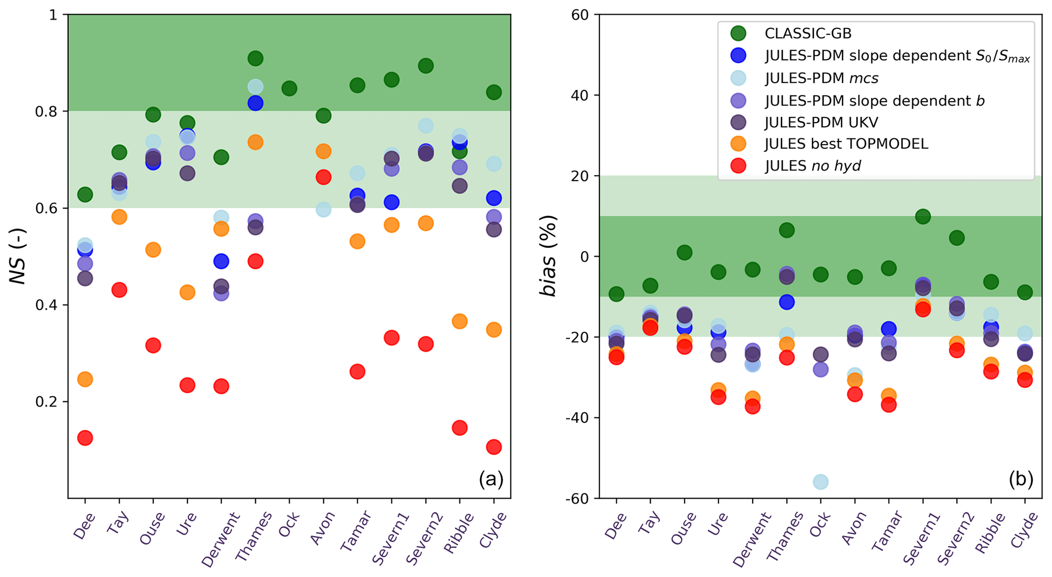
Figure 8River flow performance metrics for catchment tests: green is the CLASSIC-GB model (Crooks et al., 2014), blue is JULES using the PDM parameters detailed in Sect. 3.4 (fixed b=2.0 and grid-cell slope-dependent S0∕Smax), light blue is JULES using PDM parameters following mcs criterion in Sect. 3.3 (fixed b=2.0 and mean catchment slope-dependent S0∕Smax), slate blue is JULES using PDM parameters of grid-cell slope-dependent b (Sect. 2.2.2) and fixed S0/Smax=0.0, dark blue is JULES using PDM parameters defined in the UKV configuration (b=0.4, S0/Smax=0.0), orange is JULES using the TOPMODEL scheme with the parameters obtained by the best-performing results (α=1, f=5.0), red is JULES using no saturation excess scheme to produce runoff (no hyd). (a) NS efficiency. (b) Mean bias. Background plot colours indicate the performance category: green is category 1, light green is category 2 and white is category 3.
We have additionally carried out simulations where both hydrology schemes PDM and TOPMODEL are switched off (no hyd runs, red markers in Fig. 8), where surface runoff can only be generated by infiltration excess (Hortonian runoff). The metrics for this no hyd simulations are very low (mostly under category 3) due to a low surface runoff generation and little accuracy in the timing of the baseflow discharge (subsurface runoff through the simple free drainage approach comes in late; Fig. 9). The infiltration excess surface runoff is rarely invoked in JULES as the rate of water reaching the surface at each time step does not reach the maximum infiltration rate, which is defined as the saturation conductivity at the upper soil layer enhanced by a land cover factor (Best et al., 2011; Clark et al., 2011). This issue has been reported before for the JULES model (Clark and Gedney, 2008) and other LSMs (Balsamo et al., 2009; Boone et al., 2004).
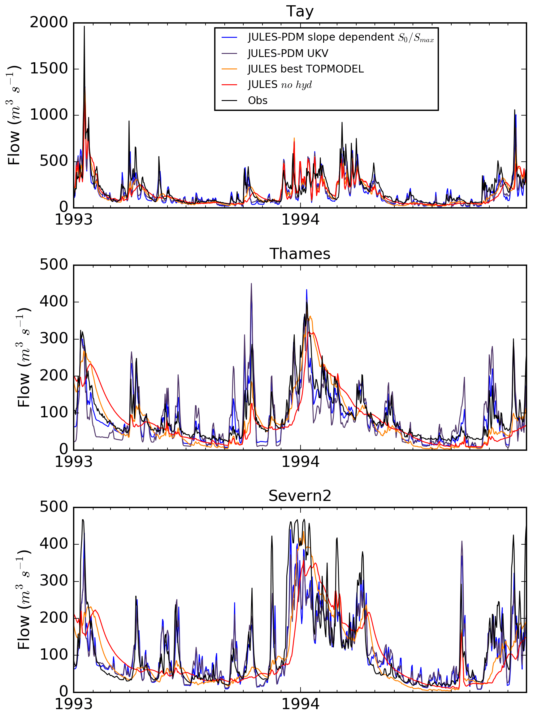
Figure 9Daily river flow (1993–1994) for the three larger catchments studied: Tay, Thames and Severn2 (Fig. 1). Observations at the NRFA gauge station (Table 1) are in black. Simulations at the outlet grid by JULES are shown: using the PDM parameters detailed in Sect. 3.4 (fixed b=2.0 and grid-cell slope-dependent S0∕Smax) in blue, using PDM parameters defined in the UKV configuration (b=0.4, S0/Smax=0.0) in dark blue, using TOPMODEL scheme with the parameters that obtained the best-performing results (α=1, f=5.0) in orange, and using no saturation excess scheme to produce runoff (no hyd) in red.
The TOPMODEL tests results using the parameters that best fit the observations out of all tests detailed in Sect. 2.2.2 (α=1, f=5.0) are also represented in Fig. 8 (orange markers). Although the bias shows very little improvement from the no hyd runs due to a low estimation of surface runoff, the NS metric shows an improvement in all catchments, as the surface runoff production by saturation excess is active and the rainfall peaks do produce river flow peaks. The baseflow production during dry periods is not as delayed as it is in the no hyd runs (Fig. 9). However, only the Thames and the Avon reach category 2 in terms of NS performance when using TOPMODEL.
The markers in different shades of blue in Fig. 8 represent JULES simulations using the PDM scheme. As a representation of the state-of-the-art parameterisation for UK hydrology using JULES at the Met Office, we include in this comparison the PDM tests using a grid-cell slope-dependent b parameter as defined in Sect. 2.2.2 (slate-blue markers) and the tests using b=0.4 and S0/Smax=0.0 (dark blue), which are the PDM parameters from the Met Office operational weather forecast UK science configuration (UKV; e.g. Tang et al., 2013). These two sets of tests reach a very similar performance for all catchments, improving the mean bias of the TOPMODEL tests as higher surface runoff is generated during rainfall events and also consistently improving the NS metric and reaching the category 2 performance for most catchments. However, over the baseflow-dominated catchments Thames, Derwent and Avon, these PDM parameterisations are still in category 3 in terms of NS performance and were outperformed by the TOPMODEL tests. This is mostly due to exceedingly “flashy” daily time series of river flow during rainfall events and consequently low baseflow due to drainage through the bottom of the soil column during drier periods, as the soil did not get wet enough during the previous wet episodes. The inclusion of the mean catchment terrain slope dependency on the S0/Smax parameter using the mcs criterion (light blue markers) clearly improves the performance from the rest of the tests (except in the Avon catchment), showing how we now include an appropriate characterisation, not only for flashy catchments on steeper terrain (Dee, Ribble, Severn1–2, Tay; see Fig. 9), but also for flatter catchments where PDM is typically outperformed by TOPMODEL (Thames, Derwent). This improvement in flatter catchments is due to a constraint in the surface runoff production during rainfall spells introduced by the S0/Smax parameter: improving the timing of the baseflow production during dry periods since the soil keeps memory from wet periods when not every rainfall event could produce surface runoff. Finally, the simulations using a linear dependency on grid-cell slope for the S0/Smax parameter as detailed in Sect. 3.4 (blue markers) lose some of the predictive skill in the mcs tests, but improve the rest of tests overall, reaching the category 1 NS performance for the Thames catchment (Fig. 9) and category 2 for most of the rest.
3.6 Performance on non-daily timescales
Simulated river flows using LSMs will result from physical processes represented in the model and the imposed meteorological driving data. Both of these factors affect the simulations on a range of different timescales. We have used cross-spectral analysis to investigate the implications of the final parameterisation using grid-slope dependency for S0/Smax beyond the evaluations using the mean bias error and Nash–Sutcliffe efficiency assessed on the daily timescale. In particular, this allows assessment of the average amplitude of discharge on different timescales and, separately, the average phase difference (lead or lag) of the modelled compared to the observed discharge (Weedon et al., 2015). The timescales investigated cross spectrally range from 2 days to the length of the time series or 10 years. The ideal model performance at a particular frequency leads to an amplitude ratio of exactly 1.0 or a result with 95 % confidence intervals (CIs) that overlap 1.0. For clarity in Figs. 10 and 11, we illustrate amplitude ratios rather than decibels used in engineering. In terms of phase difference an ideal result at a particular frequency would be variations “in phase” (phase difference of exactly 0.0∘ or value with 95 % CIs overlapping 0∘). Here positive phase differences mean that the model variations lag behind the observations and negative values indicate the model leading the observations.
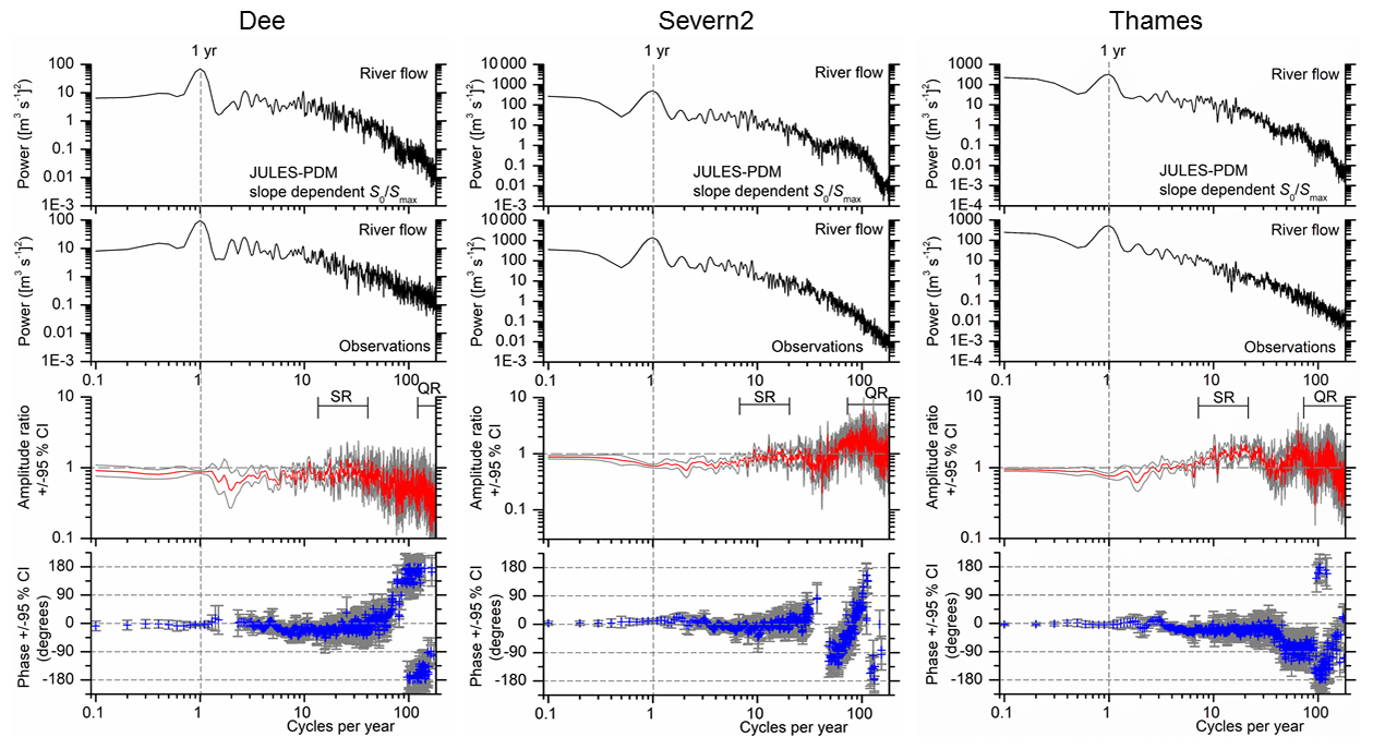
Figure 10Cross-spectral analysis of river flow from JULES-PDM using slope-dependent S0/Smax for three catchments: Dee (left), Severn2 (middle) and Thames (right). In each case the variability and relative timing of daily JULES output river flow is assessed against the daily observed river flow for a range of frequencies (spanning 10 years on the left to 2 days on the right of the spectra). For each catchment the top two panels show the power or variance spectra. In the form of spectral analysis applied here the power directly indicates the mean squared amplitude at each frequency (rather than the area under the plot; Weedon et al., 2015). The ideal model performance results in amplitude ratios (third row) indistinguishable from 1.0 and phase differences (bottom row) indistinguishable from 0.0. Theoretical phase-difference trends are shown with black dashed lines (bottom row). The amplitude ratio is shown as a red line with the grey lines above and below showing the 95 % confidence interval. Phase differences are shown as blue crosses, but only at frequencies where the coherency between series exceeds the 95 % confidence level (Weedon et al., 2015). The 95 % confidence intervals associated with the phase differences are indicated using vertical grey bars.
Cross-spectral analysis of the JULES performance on different timescales has been carried out for the final parameterisation using grid-slope dependency for S0/Smax for three catchments representative of different topographical characteristics (Dee, Severn2 and Thames). Note that the JULES discharge performance was assessed against observations with cross-spectral analysis by Weedon et al. (2015) but the model was run at daily time steps, which caused numerical artefacts in discharge variability (excessive high-frequency attenuation). Here RFM routing was applied subdaily, thereby avoiding the artefacts. The timescales on which amplitude ratios and phase differences have been assessed are annual, slow-response scale (SR) and quick-response scale (QR). The upper limits of the SR and QR timescales are determined for each catchment as the time that river flow takes to flow from the upper most point of the catchment to the outlet, using the wave speeds that RFM uses in JULES for subsurface and surface flow, respectively. The lower limits of the timescales are defined as one-third of the upper limits. The SR and QR timescales for the three catchments analysed are shown in Table 3. Results of the cross-spectral analysis of the daily river flow (power spectra, amplitude ratio spectrum and phase difference or phase spectrum) are shown in Fig. 10. If a time series is compared to itself, but offset by a few time steps, there is a resulting trend in the high-frequency part of the phase-difference spectrum (Eq. A10 in Weedon et al., 2015). The modelled phase-difference trends that approximate the results are shown using black dashed lines in Fig. 10. Note that phase differences distinguishable from zero degrees can result from both simple offsets in the timing of model output compared to the observations (causing phase-difference trends) and from incorrect modelling of the response times of hydrological stores (Weedon et al., 2015).
Table 3SR (slow response) and QR (quick response) timescales for the cross-spectral analysis conducted at three catchments in Sect. 3.6.
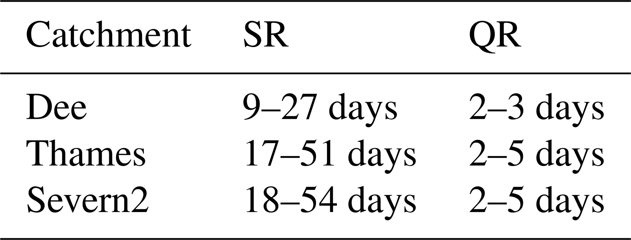
A further comparison between amplitude and phase differences with observations using different parameterisations and on different timescales helps to clarify the implications of our final parameterisation and model development (Fig. 11). The annual-scale spectral peak is very marked in the wet northern Dee catchment, and all flavours of JULES represented capture it accurately (amplitude ratios are close to 1.0 allowing for the 95 % CIs). However, in the Severn2 and Thames catchments we start to see compromised performances on the annual scale. The best TOPMODEL tests outperform the rest for both catchments, even though the final parameterisation (slope-dependent S0/Smax) presents good results in terms of amplitude ratio (0.60±0.04 and 0.76±0.07, respectively) and phase difference (10.7∘ ± 5.75∘ and −4.4∘ ± 7.7∘).
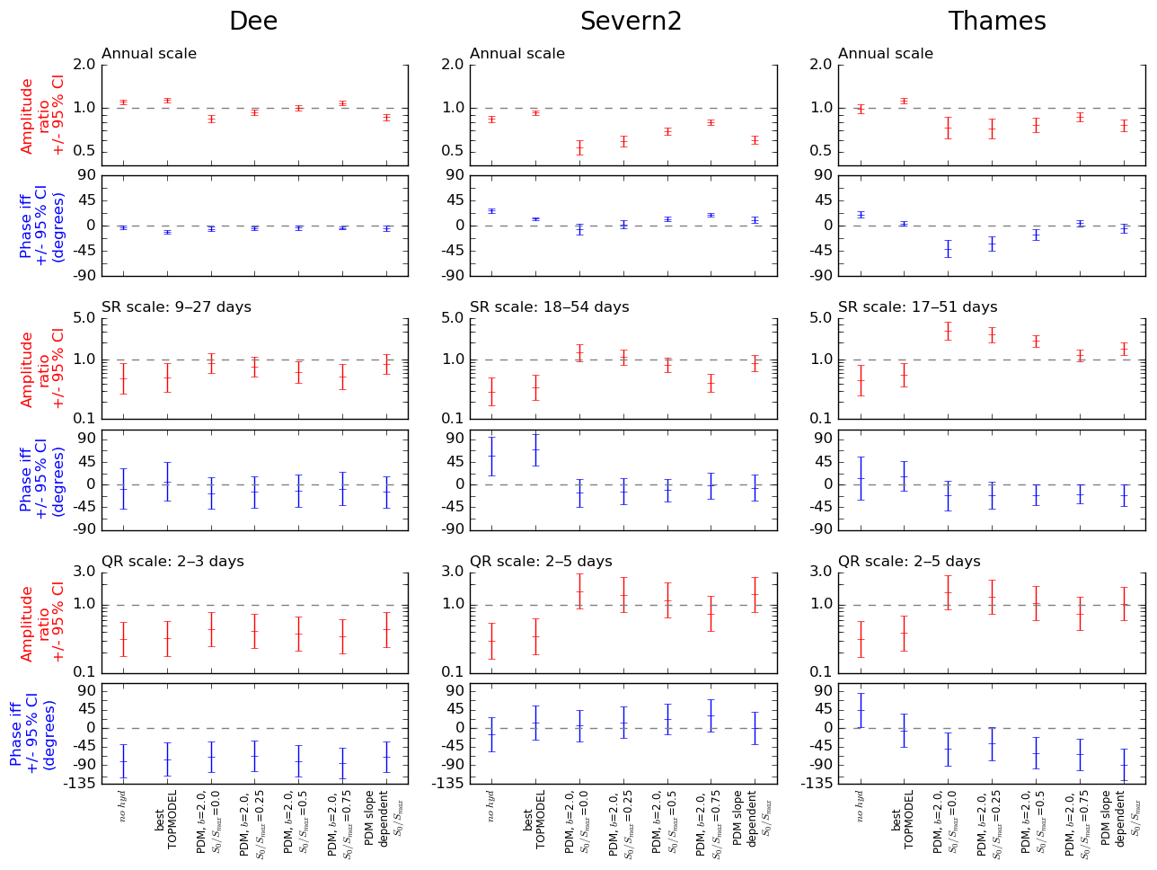
Figure 11Cross-spectral analysis of river flow from JULES using a range of parameterisations from the tests described in Sect. 2.2.2, for three catchments: Dee (left), Severn2 (middle) and Thames (right). From left to right on the x axis of every plot: no hyd (as in Figs. 8–9), best TOPMODEL (as in Figs. 8–9), PDM with b=2.0 and S0/Smax=0.0, PDM with b=2.0 and S0/Smax=0.25, PDM with b=2.0 and S0/Smax=0.5, PDM with b=2.0 and S0/Smax=0.75 and PDM with b=2.0 and grid-cell slope-dependent S0∕Smax (as in Figs. 8–9). For each catchment, amplitude ratios (red) and phase differences (blue) are shown on the annual scale (top two rows), SR scale (middle two rows) and QR scale (bottom two rows).
On the SR scale the results agree with the findings using an NS metric for the three catchments; the new parameterisation results are close to 0∘ for phase difference, allowing for their 95 % CIs, and close to 1.0 for the amplitude ratio with the exception of the Thames catchment, where the amplitude ratio of 1.57 (95 % CI: 1.23 to 2.01) is only outperformed by the parameterisation using the mcs criterion. On the QR scale we expected results to resemble the NS metric analysis, and we find that over the three catchments the new parameterisation results are the best or as good as the mcs criterion results as seen in Sect. 3.4 and 3.5, with the exception of a lead in discharge for the Thames catchment that is apparently higher than that of the rest of the PDM tests.
The cross-spectral results illustrated in Figs. 10 and 11 demonstrate that, despite the marked improvement in model performance when utilising the new parameterisation judged using NS and bias, there remains scope for further improvements on multi-day to annual timescales.
To our knowledge, this is the first study that analyses river flow model outputs from a LSM over a wide enough area (the 13 selected catchments) driven by the CHESS-met dataset (Robinson et al., 2017a, b). The availability of this dataset opens new possibilities to study land surface hydrology and interactions with the atmosphere using LSMs (that typically require gridded forcing datasets) on the kilometre scale driven by gridded rainfall derived from gauge stations. A recent study (Blyth et al., 2019) investigates evapotranspiration trends and components in Great Britain over the last 55 years using CHESS-met and the JULES runoff development described in this paper. These authors find that, when compared to flux tower data, the model overestimates evapotranspiration rates. Excesses of evaporation by JULES have also been reported on the global scale (Schellekens et al., 2017) and using eddy covariance flux measurements in temperate Europe (Van den Hoof et al., 2013). The sources of this evaporation bias are beyond the scope of this work and other studies in the model community are investigating the issue (e.g. Blyth et al., 2019). However, the new runoff development reduces the negative runoff bias as shown here, mostly from increased surface runoff during the rainy season over mountainous regions. Hence, the evapotranspiration rates in the Blyth et al. (2019) study have been impacted in the right direction. Knowing whether this reduction in evapotranspiration in Great Britain by lower soil moisture availability is consistent with soil moisture observations remains a challenge. We anticipate that this could be approached using a UK network of appropriate data for area-integrated soil moisture currently being developed (COSMOS-UK: https://cosmos.ceh.ac.uk, last access: 13 February 2019).
We acknowledge that topographic variability on the grid scale is not new to JULES or other LSMs, as it is considered by the TOPMODEL scheme. However, we have found that for regional integration in Great Britain the surface runoff production by PDM allows for a better characterisation of the topographical variability through the S0 parameter. This finding within the JULES model and the regional framework of Great Britain can have significant impacts over other regions and be applied to other models that need to account for subgrid variability in the runoff generation process, using a widely available parameter (from digital elevation model datasets) like the grid-cell mean slope as the only input, whereas other physical characteristics might be more difficult to obtain or are simply unavailable.
The poor performance at the Avon catchment by the PDM scheme has not been solved by our new parameterisation, pointing to geological rather than topographical characteristics driving the subsurface water flow (Rahman and Rosolem, 2017). We argue that a combination of the PDM scheme for surface runoff generation and TOPMODEL, or another scheme that incorporates the representation of groundwater dynamics and persistence at the subsurface (e.g. Fan et al., 2007; Miguez-Macho et al., 2007), should be the way forward for JULES developments.
We stress that the issue of the infiltration excess surface runoff rarely being invoked in JULES needs to be further investigated (e.g. Mueller et al., 2016; Largeron et al., 2018). The maximum infiltration rate that will produce surface runoff is theoretically reached from sudden and intense rainfall events. Such a rate is difficult to reach by LSMs, since they are currently driven by precipitation datasets that lack the temporal and spatial resolution necessary to correctly represent intense rainfall events (Balsamo et al., 2009; Boone et al., 2004; Clark and Gedney, 2008). The saturation excess surface runoff is overwhelmingly dominant in this study and might be compensating for underestimations of infiltration excess.
The performance loss when using grid-slope dependency instead of mean catchment slope dependency is a compromise that we accept since our development and recommended configuration need to be applicable for the whole of Great Britain and even for other regions and space scales where particular catchment information might not be available.
The JULES model does not incorporate anthropogenic effects on river flow in its current state. We acknowledge that human activities (groundwater abstractions, dams, reservoirs) affect the observed river flow in Great Britain and therefore JULES outputs of natural river flow are not expected to exactly reproduce the observed NRFA records. As mentioned in Sect. 2.2.2, we included the naturalised flow records for the Thames catchment as it is the only catchment with natural flow availability for the studied period. However, the effects of human activities on river flow are difficult to quantify given the lack of data and heterogeneity of activities in the studied catchments. A recent study over Great Britain, for instance, showed an increase in drought duration in catchments affected by groundwater abstractions and varying effects on drought occurrence depending on the activities (Tijdeman et al., 2018).
The model development described here on the kilometre scale and over the domain of Great Britain is based on the inclusion of a terrain slope dependency in the soil wetness parameter that switches on the saturation excess runoff scheme. Even though the parameter values need to be re-examined for other regions and resolutions, this physical dependency should also be valid on the global scale and its implications in the performance of the JULES model global simulations at 0.25 and 0.5∘ of spatial resolution are being evaluated in the EartH2Observe programme (Schellekens et al., 2017).
Motivated by the search for the best representation of hydrological processes over the land in the context of a coupled UK land–ocean–atmosphere model (UKC2; Lewis et al., 2018), we find that the JULES LSM has the potential to simulate daily river flow accurately over selected catchments in Great Britain when driven by the 1 km2 resolution CHESS-met database, obtaining results comparable to those of a rainfall-runoff model for Great Britain (CLASSIC-GB, Crooks et al., 2014). Previous studies using JULES (e.g. Best et al., 2015; Schellekens et al., 2017; Ukkola et al., 2016) use a fixed S0 parameter within the PDM scheme. In this study we vary the values of S0 and are able to improve performance (% bias and NS) as a result. The parameter S0 controls the soil water content necessary to start producing surface runoff.
The parameterisation that produces the best results for each catchment uses the mean catchment slope. When applied to a gridded model, a new linear function of slope on the model resolution scale can produce performance metrics comparable to those using the mean catchment slope. The new parameterisation constrains surface runoff production to wet soil conditions over flatter regions, whereas over steeper regions the model produces surface runoff for every rainfall event, regardless of the soil wetness conditions.
Hence, a simple terrain slope dependency has greatly improved the JULES river flow results for different catchments in Great Britain. We stress that this finding should be tested for other regions and scales on JULES and other LSMs, as topography datasets are available at very fine resolution (e.g. http://www.hydrosheds.org/, last access: 13 February 2019). The capability of an LSM to reproduce the water balance on regional scales with a performance (in terms of river flow generation) comparable to that of hydrological models can potentially impact weather forecast and climate predictions using regional coupled modelling systems such as UKC2.
We have also shown that cross-spectral analysis for evaluating model performance against observations quantifies the mismatches in variability and separately mismatches in phase at different timescales that are not otherwise apparent from metrics such as NS and RMSE. Potentially, the recognition of a specific timescale on which a model is performing poorly could help to identify the incorrect behaviour in terms of water transport and/or subsurface storage. The cross-spectral analysis comparing the modelled river flow with observations has reinforced the choice of the new parameterisation for surface runoff production.
Model development
The work presented here has led to a JULES code development that introduces the capability of using S0/Smax as a model parameter, either as a fixed value or as a grid-cell slope-dependent value, as well as the capability to read in the model grid topographic slope as an ancillary dataset. The new version of the model with the new parameterisation recommended here has been used to study evaporation and water budgets in Great Britain during the last 55 years by Blyth et al. (2019), producing outputs that are publicly available: the CEH CHESS-land dataset (Martínez-de la Torre et al., 2018). The development is also incorporated into the UKC2 system (Lewis et al., 2018). The new code development is described in ticket no. 262 of the JULES FCM repository (https://code.metoffice.gov.uk/trac/jules/, last access: 13 February 2019), and has become part of the JULES trunk since the version 4.9 release.
This study uses JULES revision 1709, which is between the 4.3 and 4.4 releases. The code can be downloaded from the JULES FCM repository at https://code.metoffice.gov.uk/trac/jules/ (last access: 13 February 2019, registration required).
JULES LSM output data for this work are available from the corresponding author upon request. The river flow observations at gauging stations used here were facilitated by NRFA and are publicly available (http://nrfa.ceh.ac.uk/, last access: 13 February 2019). The CHESS-met driving data and the rest of the ancillary datasets used here are publicly available through references given in Sect. 2.2.1.
EMB and AMdlT initially designed the experiments. AMdlT ran the model simulations, designed and performed the model developments and carried out the analysis of results. GPW contributed the design and performance of cross-spectral analysis in Sect. 3.6. AM wrote the initial draft of the paper and all authors contributed to the final written version.
The authors declare that they have no conflict of interest.
This research has been carried out under national capability funding as part
of a directed effort on UK Environmental Prediction (UKEP), a collaboration
project between Centre for Ecology & Hydrology (CEH), the Met Office,
National Oceanography Centre (NOC) and Plymouth Marine Laboratory
(PML).
Edited by: Wolfgang
Kurtz
Reviewed by: two anonymous referees
Balsamo, G., Beljaars, A., Scipal, K., Viterbo, P., van den Hurk, B., Hirschi, M., and Betts, A. K.: A Revised Hydrology for the ECMWF Model: Verification from Field Site to Terrestrial Water Storage and Impact in the Integrated Forecast System, J. Hydrometeorol., 10, 623–643, https://doi.org/10.1175/2008jhm1068.1, 2009.
Bastola, S., Murphy, C., and Sweeney, J.: The role of hydrological modelling uncertainties in climate change impact assessments of Irish river catchments, Adv. Water Resour., 34, 562–576, https://doi.org/10.1016/j.advwatres.2011.01.008, 2011.
Beck, H. E., van Dijk, A. I., de Roo, A., Miralles, D. G., McVicar, T. R., Schellekens, J., and Bruijnzeel, L. A.: Global-scale regionalization of hydrologic model parameters, Water Resour. Res., 52, 3599–3622, https://doi.org/10.1002/2015WR018247, 2016.
Bell, V. A., Kay, A. L., Jones, R. G., and Moore, R. J.: Development of a high resolution grid-based river flow model for use with regional climate model output, Hydrol. Earth Syst. Sci., 11, 532–549, https://doi.org/10.5194/hess-11-532-2007, 2007.
Best, M. J., Pryor, M., Clark, D. B., Rooney, G. G., Essery, R. L. H., Ménard, C. B., Edwards, J. M., Hendry, M. A., Porson, A., Gedney, N., Mercado, L. M., Sitch, S., Blyth, E., Boucher, O., Cox, P. M., Grimmond, C. S. B., and Harding, R. J.: The Joint UK Land Environment Simulator (JULES), model description – Part 1: Energy and water fluxes, Geosci. Model Dev., 4, 677–699, https://doi.org/10.5194/gmd-4-677-2011, 2011.
Best, M. J., Abramowitz, G., Johnson, H. R., Pitman, A. J., Balsamo, G., Boone, A., Cuntz, M., Decharme, B., Dirmeyer, P. A., Dong, J., Ek, M., Guo, Z., Haverd, V., van den Hurk, B. J. J., Nearing, G. S., Pak, B., Peters-Lidard, C., Santanello Jr., J. A., Stevens, L., and Vuichard, N.: The Plumbing of Land Surface Models: Benchmarking Model Performance, J. Hydrometeorol., 16, 1425–1442, https://doi.org/10.1175/jhm-d-14-0158.1, 2015.
Betts, R.: Implications of land ecosystem-atmosphere interactions for strategies for climate change adaptation and mitigation, Tellus B, 59, 602–615, https://doi.org/10.1111/j.1600-0889.2007.00284.x, 2007.
Beven, K. J. and Kirkby, M. J.: A physically based, variable contributing area model of basin hydrology/Un modèle à base physique de zone d'appel variable de l'hydrologie du bassin versant, Hydrol. Sci. B., 24, 43–69, https://doi.org/10.1080/02626667909491834, 1979.
Blyth, E.: Modelling soil moisture for a grassland and a woodland site in south-east England, Hydrol. Earth Syst. Sci., 6, 39–48, https://doi.org/10.5194/hess-6-39-2002, 2002.
Blyth, E., Clark, D. B., Ellis, R., Huntingford, C., Los, S., Pryor, M., Best, M., and Sitch, S.: A comprehensive set of benchmark tests for a land surface model of simultaneous fluxes of water and carbon at both the global and seasonal scale, Geosci. Model Dev., 4, 255–269, https://doi.org/10.5194/gmd-4-255-2011, 2011.
Blyth, E. M., Martínez-de la Torre, A., and Robinson, E. L.: Trends in evapotranspiration and its drivers in Great Britain: 1961 to 2015, Prog. Phys. Geog., in review, 2019.
Boone, A., Habets, F., Noilhan, J., Clark, D., Dirmeyer, P., Fox, S., Gusev, Y., Haddeland, I., Koster, R., Lohmann, D., Mahanama, S., Mitchell, K., Nasonova, O., Niu, G.-Y., Pitman, A., Polcher, J., Shmakin, A.B., Tanaka, K., van den Hurk, B., Vérant, S., Verseghy, D., Viterbo, P., and Yang, Z.-L.: The Rhône-Aggregation Land Surface Scheme Intercomparison Project: An Overview, J. Climate, 17, 187–208, https://doi.org/10.1175/1520-0442(2004)017<0187:trlssi>2.0.co;2, 2004.
Boorman, D. B., Hollis, J. M., and Lilly, A.: Hydrology of soil types: a hydrologically-based classification of the soils of United Kingdom, Wallingford, Institute of Hydrology, IH Report no.126, 146 pp., 1995.
Brooks, R. H. and Corey, A. T.: Hydraulic properties of porous media, Hydrology Papers, Colorado State University, 1964.
Campoy, A., Ducharne, A., Cheruy, F., Hourdin, F., Polcher, J., and Dupont, J. C.: Response of land surface fluxes and precipitation to different soil bottom hydrological conditions in a general circulation model, J. Geophys. Res.-Atmos., 118, 10725–10739, https://doi.org/10.1002/jgrd.50627, 2013.
Chen, J. and Kumar, P.: Topographic Influence on the Seasonal and Interannual Variation of Water and Energy Balance of Basins in North America, J. Climate, 14, 1989–2014, https://doi.org/10.1175/1520-0442(2001)014<1989:tiotsa>2.0.co;2, 2001.
Clark, D. B. and Gedney, N.: Representing the effects of subgrid variability of soil moisture on runoff generation in a land surface model. J. Geophys. Res.-Atmos., 113, D10111, https://doi.org/10.1029/2007JD008940, 2008.
Clark, D. B., Mercado, L. M., Sitch, S., Jones, C. D., Gedney, N., Best, M. J., Pryor, M., Rooney, G. G., Essery, R. L. H., Blyth, E., Boucher, O., Harding, R. J., Huntingford, C., and Cox, P. M.: The Joint UK Land Environment Simulator (JULES), model description – Part 2: Carbon fluxes and vegetation dynamics, Geosci. Model Dev., 4, 701–722, https://doi.org/10.5194/gmd-4-701-2011, 2011.
Clark, M. P., Fan, Y., Lawrence, D. M., Adam, J. C., Bolster, D., Gochis, D. J., Hooper, R. P., Kumar, M., Leung, L. R., Mackay, D. S., Maxwell, R. M., Shen, C., Swenson, S. C., and Zeng, X.: Improving the representation of hydrologic processes in Earth System Models, Water Resour. Res., 51, 5929–5956, https://doi.org/10.1002/2015WR017096, 2015.
Cosby, B. J., Hornberger, G. M., Clapp, R. B., and Ginn, T. R.: A Statistical Exploration of the Relationships of Soil Moisture Characteristics to the Physical Properties of Soils, Water Resour. Res., 20, 682–690, https://doi.org/10.1029/WR020i006p00682, 1984.
Cox, P. M., Betts, R. A., Bunton, C. B., Essery, R. L. H., Rowntree, P. R., and Smith, J.: The impact of new land surface physics on the GCM simulation of climate and climate sensitivity, Clim. Dynam., 15, 183–203, https://doi.org/10.1007/s003820050276, 1999.
Crooks, S., Kay, A., Davies, H., and Bell, V.: From Catchment to National Scale Rainfall-Runoff Modelling: Demonstration of a Hydrological Modelling Framework, Hydrology, 1, 63–88, https://doi.org/10.3390/hydrology1010063, 2014.
Davies, H. N. and Bell, V. A.: Assessment of methods for extracting low-resolution river networks from high-resolution digital data, Hydrolog. Sci. J., 54, 17–28, https://doi.org/10.1623/hysj.54.1.17, 2009.
Dharssi, I., Vidale, P. L., Verhoef, A., Macpherson, B., Jones, C. D., and Best, M.: New soil physical properties implemented in the Unified Model at PS18, Met Office, Exeter, Met Office Technical Report No. 528, 2009.
Fan, Y., Miguez-Macho, G., Weaver, C. P., Walko, R., and Robock, A.: Incorporating water table dynamics in climate modeling: 1. Water table observations and equilibrium water table simulations, J. Geophys. Res.-Atmos., 112, D10125, https://doi.org/10.1029/2006JD008111, 2007.
FAO/IIASA/ISRIC/ISS-CAS/JRC: Harmonized World Soil Database (version 1.2), FAO, Rome, Italy and IIASA, Laxenburg, Austria, 2012.
Farrant, A. R. and Cooper, A. H.: Karst geohazards in the UK: the use of digital data for hazard management, Q. J. Eng. Geol. Hydroge., 41, 339–356, https://doi.org/10.1144/1470-9236/07-201, 2008.
Finney, D. L., Blyth, E., and Ellis, R.: Improved modelling of Siberian river flow through the use of an alternative frozen soil hydrology scheme in a land surface model, The Cryosphere, 6, 859–870, https://doi.org/10.5194/tc-6-859-2012, 2012.
Fuller, R. M., Smith, G. M., Sanderson, J. M., Hill, R. A., and Thomson, A. G.: The UK Land Cover Map 2000: Construction of a Parcel-Based Vector Map from Satellite Images, Cartogr. J., 39, 15–25, https://doi.org/10.1179/caj.2002.39.1.15, 2002.
Gedney, N. and Cox, P. M.: The Sensitivity of Global Climate Model Simulations to the Representation of Soil Moisture Heterogeneity, J. Hydrometeorol., 4, 1265–1275, https://doi.org/10.1175/1525-7541(2003)004<1265:tsogcm>2.0.co;2, 2003.
Gudmundsson, L., Tallaksen, L. M., Stahl, K., Clark, D. B., Dumont, E., Hagemann, S., Bertrand, N., Gerten, D., Heinke, J., Hanasaki, N., Voss, F., and Koirala, S.: Comparing Large-Scale Hydrological Model Simulations to Observed Runoff Percentiles in Europe, J. Hydrometeorol., 13, 604–620, https://doi.org/10.1175/jhm-d-11-083.1, 2012.
Harrison, R. G., Jones, C. D., and Hughes, J. K.: Competing roles of rising CO2 and climate change in the contemporary European carbon balance, Biogeosciences, 5, 1–10, https://doi.org/10.5194/bg-5-1-2008, 2008.
Horn, B. K. P.: Hill Shading and the Reflectance Map, P. IEEE, 69, 14–47, https://doi.org/10.1109/Proc.1981.11918, 1981.
Hough, M. N. and Jones, R. J. A.: The United Kingdom Meteorological Office rainfall and evaporation calculation system: MORECS version 2.0 – an overview, Hydrol. Earth Syst. Sci., 1, 227–239, https://doi.org/10.5194/hess-1-227-1997, 1997.
Keller, V. D. J., Tanguy, M., Prosdocimi, I., Terry, J. A., Hitt, O., Cole, S. J., Fry, M., Morris, D. G., and Dixon, H.: CEH-GEAR: 1 km resolution daily and monthly areal rainfall estimates for the UK for hydrological and other applications, Earth Syst. Sci. Data, 7, 143–155, https://doi.org/10.5194/essd-7-143-2015, 2015.
Largeron, C., Cloke, H., Verhoef, A., Martínez-de la Torre, A., and Mueller, A.: Impact of the representation of the infiltration on the river flow during intense rainfall events in Jules, ECMWF, Reading, Technical Memorandum 821, ECMWF, https://doi.org/10.21957/nkky9s1hs, 2018.
Lewis, H. W., Castillo Sanchez, J. M., Graham, J., Saulter, A., Bornemann, J., Arnold, A., Fallmann, J., Harris, C., Pearson, D., Ramsdale, S., Martínez-de la Torre, A., Bricheno, L., Blyth, E., Bell, V. A., Davies, H., Marthews, T. R., O'Neill, C., Rumbold, H., O'Dea, E., Brereton, A., Guihou, K., Hines, A., Butenschon, M., Dadson, S. J., Palmer, T., Holt, J., Reynard, N., Best, M., Edwards, J., and Siddorn, J.: The UKC2 regional coupled environmental prediction system, Geosci. Model Dev., 11, 1–42, https://doi.org/10.5194/gmd-11-1-2018, 2018.
Marthews, T. R., Quesada, C. A., Galbraith, D. R., Malhi, Y., Mullins, C. E., Hodnett, M. G., and Dharssi, I.: High-resolution hydraulic parameter maps for surface soils in tropical South America, Geosci. Model Dev., 7, 711–723, https://doi.org/10.5194/gmd-7-711-2014, 2014.
Marthews, T. R., Dadson, S. J., Lehner, B., Abele, S., and Gedney, N.: High-resolution global topographic index values for use in large-scale hydrological modelling, Hydrol. Earth Syst. Sci., 19, 91–104, https://doi.org/10.5194/hess-19-91-2015, 2015.
Martínez-de la Torre, A., Blyth, E. M., and Robinson, E. L.: Water, carbon and energy fluxes simulation for Great Britain using the JULES Land Surface Model and the Climate Hydrology and Ecology research Support System meteorology dataset (1961–2015) [CHESS-land], NERC Environmental Information Data Centre, UK, https://doi.org/10.5285/c76096d6-45d4-4a69-a310-4c67f8dcf096, 2018.
Miguez-Macho, G., Fan, Y., Weaver, C. P., Walko, R., and Robock, A.: Incorporating water table dynamics in climate modeling: 2. Formulation, validation, and soil moisture simulation. J. Geophys. Res.-Atmos., 112, D13108, https://doi.org/10.1029/2006JD008112, 2007.
Mizukami, N., Clark, M. P., Newman, A. J., Wood, A. W., Gutmann, E. D., Nijssen, B., Rakovec, O., and Samaniego, L.: Towards seamless large-domain parameter estimation for hydrologic models, Water Resour. Res., 53, 8020–8040, https://doi.org/10.1002/2017WR020401, 2017.
Moore, R. J.: The probability-distributed principle and runoff production at point and basin scales, Hydrolog. Sci. J., 30, 273–297, https://doi.org/10.1080/02626668509490989, 1985.
Moore, R. J.: The PDM rainfall-runoff model, Hydrol. Earth Syst. Sci., 11, 483–499, https://doi.org/10.5194/hess-11-483-2007, 2007.
Morris, D. G. and Flavin, R. W.: A digital terrain model for hydrology, Proc. 4th International Symposium on Spatial Data Handling, 23–27 July, Zürich, Vol. 1, 250–262, 1990.
Morris, D. G. and Flavin, R. W.: Sub-set of UK 50 m by 50 m hydrological digital terrain model grids, NERC Institute of Hydrology Wallingford, 1994.
Mueller, A., Dutra, E., Cloke, H., Verhoef, A., Balsamo, G., and Pappenberger, F.: Water infiltration and redistribution in Land Surface Models, ECMWF, Reading, Technical Memorandum 791, ECMWF, https://doi.org/10.21957/ppksejqu9, 2016.
Nash, J. E. and Sutcliffe, J. V.: River flow forecasting through conceptual models part I – A discussion of principles, J. Hydrol., 10, 282–290, https://doi.org/10.1016/0022-1694(70)90255-6, 1970.
Niu, G.-Y. and Yang, Z.-L.: The versatile integrator of surface atmospheric processes: Part 2: evaluation of three topography-based runoff schemes, Global Planet. Change, 38, 191–208, https://doi.org/10.1016/S0921-8181(03)00029-8, 2003.
Oleson, K. W., Lawrence, D. M., Bonan, G. B., Flanner, M. G., Kluzek, E., Lawrence, P. J., Levis, S., Swenson, S. C., Thornton, P. E., Dai, A., Decker, M., Dickinson, R., Feddema, J., Heald, C. L., Hoffman, F., Lamarque, J.-F., Mahowald, N., Niu, G.-Y., Qian, T., Randerson, J., Running, S., Sakaguchi, K., Slater, A., Stöckli, R., Wang, A., Yang, Z.-L., Zeng, X., and Zeng, X.: Technical Description of version 4.0 of the Community Land Model (CLM), NCAR, Boulder, Colorado, Technical Note NCAR/TN-478+STR, https://doi.org/10.5065/D6FB50WZ, 2010.
Papadimitriou, L. V., Koutroulis, A. G., Grillakis, M. G., and Tsanis, I. K.: High-end climate change impact on European runoff and low flows – exploring the effects of forcing biases, Hydrol. Earth Syst. Sci., 20, 1785–1808, https://doi.org/10.5194/hess-20-1785-2016, 2016.
Papadimitriou, L. V., Koutroulis, A. G., Grillakis, M. G., and Tsanis, I. K.: The effect of GCM biases on global runoff simulations of a land surface model, Hydrol. Earth Syst. Sci., 21, 4379–4401, https://doi.org/10.5194/hess-21-4379-2017, 2017.
Paz, A. R., Collischonn, W., and Lopes da Silveira, A. L.: Improvements in large-scale drainage networks derived from digital elevation models, Water Resour. Res., 42, W08502, https://doi.org/10.1029/2005WR004544, 2006.
Prudhomme, C., Wilby, R. L., Crooks, S., Kay, A. L., and Reynard, N. S.: Scenario-neutral approach to climate change impact studies: Application to flood risk, J. Hydrol., 390, 198–209, https://doi.org/10.1016/j.jhydrol.2010.06.043, 2010.
Rahman, M. and Rosolem, R.: Towards a simple representation of chalk hydrology in land surface modelling, Hydrol. Earth Syst. Sci., 21, 459–471, https://doi.org/10.5194/hess-21-459-2017, 2017.
Robinson, E. L., Blyth, E., Clark, D. B., Comyn-Platt, E., Finch, J., and Rudd, A. C.: Climate hydrology and ecology research support system meteorology dataset for Great Britain (1961–2015) [CHESS-met] v1.2, NERC Environmental Information Data Centre, UK, https://doi.org/10.5285/b745e7b1-626c-4ccc-ac27-56582e77b900, 2017a.
Robinson, E. L., Blyth, E. M., Clark, D. B., Finch, J., and Rudd, A. C.: Trends in atmospheric evaporative demand in Great Britain using high-resolution meteorological data, Hydrol. Earth Syst. Sci., 21, 1189–1224, https://doi.org/10.5194/hess-21-1189-2017, 2017b.
Schellekens, J., Dutra, E., Martínez-de la Torre, A., Balsamo, G., van Dijk, A., Sperna Weiland, F., Minvielle, M., Calvet, J.-C., Decharme, B., Eisner, S., Fink, G., Flörke, M., Peßenteiner, S., van Beek, R., Polcher, J., Beck, H., Orth, R., Calton, B., Burke, S., Dorigo, W., and Weedon, G. P.: A global water resources ensemble of hydrological models: the eartH2Observe Tier-1 dataset, Earth Syst. Sci. Data, 9, 389–413, https://doi.org/10.5194/essd-9-389-2017, 2017.
Tang, Y., Lean, H. W., and Bornemann, J.: The benefits of the Met Office variable resolution NWP model for forecasting convection, Meteorol. Appl., 20, 417–426, https://doi.org/10.1002/met.1300, 2013.
Tanguy, M., Dixon, H., Prosdocimi, I., Morris, D. G., and Keller, V. D. J.: Gridded estimates of daily and monthly areal rainfall for the United Kingdom (1890–2012) [CEH-GEAR], NERC Environmental Information Data Centre, UK, https://doi.org/10.5285/5dc179dc-f692-49ba-9326-a6893a503f6e, 2014.
Thompson, N., Barrie, I. A., Ayles, M., and Meteorological, O.: The Meteorological Office rainfall and evaporation calculation system: MORECS (July 1981), Meteorological Office, London, 1981.
Tijdeman, E., Hannaford, J., and Stahl, K.: Human influences on streamflow drought characteristics in England and Wales, Hydrol. Earth Syst. Sci., 22, 1051–1064, https://doi.org/10.5194/hess-22-1051-2018, 2018.
Ukkola, A. M., Kauwe, M. G. D., Pitman, A. J., Best, M. J., Abramowitz, G., Haverd, V., Decker, M., and Haughton, N.: Land surface models systematically overestimate the intensity, duration and magnitude of seasonal-scale evaporative droughts, Environ. Res. Lett., 11, 104012, https://doi.org/10.1088/1748-9326/11/10/104012, 2016.
Van den Hoof, C., Vidale, P. L., Verhoef, A., and Vincke, C.: Improved evaporative flux partitioning and carbon flux in the land surface model JULES: Impact on the simulation of land surface processes in temperate Europe, Agr. Forest Meteorol., 181, 108–124, https://doi.org/10.1016/j.agrformet.2013.07.011, 2013.
Van Genuchten, M. T.: A Closed-form Equation for Predicting the Hydraulic Conductivity of Unsaturated Soils, Soil Sci. Soc. Am. J., 44, 892–898, 1980.
Wagener, T. and Wheater, H. S.: Parameter estimation and regionalization for continuous rainfall-runoff models including uncertainty, J. Hydrol., 320, 132–154, https://doi.org/10.1016/j.jhydrol.2005.07.015, 2006.
Walko, R. L., Band, L. E., Baron, J., Kittel, T. G. F., Lammers, R., Lee, T. J., Ojima, D., Pielke, R. A., Taylor, C., Tague, C., Tremback, C.J. and Vidale, P.L.: Coupled Atmosphere–Biophysics–Hydrology Models for Environmental Modeling, J. Appl. Meteorol., 39, 931–944, https://doi.org/10.1175/1520-0450(2000)039<0931:cabhmf>2.0.co;2, 2000.
Weedon, G. P., Prudhomme, C., Crooks, S., Ellis, R. J., Folwell, S. S., and Best, M. J.: Evaluating the Performance of Hydrological Models via Cross-Spectral Analysis: Case Study of the Thames Basin, United Kingdom, J. Hydrometeorol., 16, 214–231, https://doi.org/10.1175/jhm-d-14-0021.1, 2015.
Williams, K. and Clark, D. B.: Disaggregation of daily data in JULES, Met Office, Exeter, 26 pp., Hadley Centre Technical Note 96, 2014.
Wösten, J. H. M., Lilly, A., Nemes, A., and Le Bas, C.: Development and use of a database of hydraulic properties of European soils, Geoderma, 90, 169–185, https://doi.org/10.1016/S0016-7061(98)00132-3, 1999.