the Creative Commons Attribution 4.0 License.
the Creative Commons Attribution 4.0 License.
 | 21 Feb 2019
A benchmark for testing the accuracy and computational cost of shortwave top-of-atmosphere reflectance calculations in clear-sky aerosol-laden atmospheres
Jeronimo Escribano
Alessio Bozzo
Philippe Dubuisson
Johannes Flemming
Robin J. Hogan
Laurent C.-Labonnote
Olivier Boucher
Accurate calculations of shortwave reflectances in clear-sky aerosol-laden atmospheres are necessary for various applications in atmospheric sciences. However, computational cost becomes increasingly important for some applications such as data assimilation of top-of-atmosphere reflectances in models of atmospheric composition. This study aims to provide a benchmark that can help in assessing these two requirements in combination. We describe a protocol and input data for 44 080 cases involving various solar and viewing geometries, four different surfaces (one oceanic bidirectional reflectance function and three albedo values for a Lambertian surface), eight aerosol optical depths, five wavelengths, and four aerosol types. We first consider two models relying on the discrete ordinate method: VLIDORT (in vector and scalar configurations) and DISORT (scalar configuration only). We use VLIDORT in its vector configuration as a reference model and quantify the loss of accuracy due to (i) neglecting the effect of polarization in DISORT and VLIDORT (scalar) models and (ii) decreasing the number of streams in DISORT. We further test two other models: the 6SV2 model, relying on the successive orders of scattering method, and Forward-Lobe Two-Stream Radiance Model (FLOTSAM), a new model under development by two of the authors. Typical mean fractional errors of 2.8 % and 2.4 % for 6SV2 and FLOTSAM are found, respectively. Computational cost depends on the input parameters but also on the code implementation and application as some models solve the radiative transfer equations for a range of geometries while others do not. All necessary input and output data are provided as a Supplement as a potential resource for interested developers and users of radiative transfer models.
- Article
(8521 KB) -
Supplement
(46898 KB) - BibTeX
- EndNote


Accurate radiative transfer calculations in the Earth's atmosphere are necessary for some applications such as remote sensing of the atmospheric and surface properties, numerical weather prediction, and climate modelling. In this study, we are interested more specifically in the calculation of radiances in the shortwave spectrum in clear-sky aerosol-laden atmospheres of the Earth for reasons explained below. Assuming perfect knowledge of the optical properties of the atmosphere and surface and a plane-parallel atmosphere, solving the radiative transfer equation is a very well posed physical problem that essentially reduces to a (not-so-easy) algorithmic and numerical problem. Accurate methods have existed for a long time, and testing the accuracy of newly developed methods has been standard practice in the radiative transfer community for some time (de Haan et al., 1987; Stamnes et al., 1988; Spurr, 2008; Kotchenova et al., 2006; Kotchenova and Vermote, 2007; Barlakas et al., 2016; Korkin et al., 2017). Well-used state-of-the-art radiative transfer models generally show agreement within 1 % (or better) under most conditions tested. There have also been a number of intercomparison or benchmarking exercises for shortwave radiance calculations, largely motivated by the requirements for accurate calculations in ground-based and satellite aerosol retrievals (Kotchenova et al., 2006; Kokhanovsky et al., 2010a; Emde et al., 2015, 2018). A classical benchmarking exercise consists of comparing the model results to well-known solutions for simple cases of a Rayleigh scattering atmosphere (Coulson et al., 1960; Natraj et al., 2009). However, such cases are very specific and do not represent the variety of conditions met in the real atmosphere. The International Polarized Radiative Transfer (IPRT) working group of the International Radiation Commission has recently defined a set of more realistic cases (Emde et al., 2015, 2018). Another benchmark is to test the numerical convergence of the scheme when the angular and/or vertical resolutions of the model are increased (de Haan et al., 1987; Ganapol, 2017). However, numerical convergence may be difficult to achieve and to assess because the numerical models may experience lower precision when the resolution is increased too much, especially for models coded in single precision. Finally, there have also been benchmarking exercises for aerosol retrievals from observed clear-sky shortwave radiances, which tests simultaneously the accuracy of the radiative transfer model and the aerosol retrieval algorithm (Kokhanovsky et al., 2010b). It should be noted that accounting for the polarization of light is necessary because it affects the accuracy of the computed radiances (e.g. Kotchenova et al., 2006) but also because some aerosol retrieval algorithms rely on the inversion of polarized radiances (e.g. Tanré et al., 2011; Dubovik et al., 2011). However, in cases where the atmosphere contains an important load of non-spherical particles (dust), errors in neglecting polarization have been reported to be less than 1 % (Barlakas, 2016).
Methods for computing shortwave radiances by solving accurately the radiative transfer equation are often computationally expensive. In data assimilation or satellite retrieval applications for which radiances have to be computed many times and on many profiles, the computational cost has always been an issue for pragmatic reasons (a numerical model that is too slow to be run on the fastest computer is virtually useless). However, developing fast or very fast radiative transfer models capable of computing radiances (and not only vertical fluxes) has received little attention so far. Exceptions include early attempts to use neural networks for fast and accurate radiative transfer in the longwave spectrum (Chevallier et al., 1998; Krasnopolsky and Chevallier, 2003; Pfreundschuh et al., 2018). It may also be possible to design fast physical algorithms in the longwave spectrum because of the weaker scattering (as compared to the shortwave spectrum) and isotropic emission (e.g. Wang et al., 2013b). In the shortwave spectrum, one can mention methods based on principal component analysis (Kopparla et al., 2017; Somkuti et al., 2017), two orders of scattering method (Natraj and Spurr, 2007), adding–doubling method (e.g. Wang et al., 2013a), or recent efforts for fast calculations of cloudy-sky visible radiances (Scheck et al., 2016). However, Scheck et al. (2016) rely on tabulated calculations (so-called lookup tables), which only allows them to consider a limited set of possible atmospheric inputs. It is noteworthy in that respect that the performance assessment of the newly released SORD (Successive ORDers of scattering) model (Korkin et al., 2017) shows a runtime analysis for the 52 benchmark cases that were tested (their Fig. 6). There is a mode in the distribution of runtimes that is below 0.01 s but also a fairly long tail with occasional runtimes between 60 and 300 s or even longer than 600 s. Finally the computational cost of algorithms for three-dimensional radiative transfer models have been investigated by Pincus and Evans (2009) and are known to be expensive.
Forecasts and reanalyses of atmospheric aerosols have been produced operationally by combining numerical models and aerosol observations in data assimilation systems (Bocquet et al., 2015; Hollingsworth et al., 2008). Aerosol information provided by satellite retrievals is often assimilated in aerosol models both in research (Collins et al., 2001) and operational (Benedetti et al., 2018) contexts. A widely assimilated quantity is the aerosol optical depth (AOD), a column-integrated quantity that quantifies the interaction of aerosols with atmospheric radiation. So far, the assimilation of AOD retrievals has been successful in constraining the model variables towards the equivalent measured variables, but as the resolution, complexity, and quality requirements of the products vary, possible inconsistencies between the assumptions used for the satellite aerosol retrieval and the model or between the different satellite retrieval algorithms arise. Furthermore, there is some information on aerosol types in the observed reflected solar radiation that may not be included in AOD products and is, therefore, lost for data assimilation.
An alternative pathway to the assimilation of AOD retrieved from passive satellite measurements is the direct assimilation of these measurements (Benedetti et al., 2018). The main challenge of doing so is basically that the satellite retrieval algorithm has to be replaced by a somehow equivalent procedure inside the data assimilation loop. In particular, a shortwave radiative transfer model (RTM) would act as a major piece of the observation operator, and some stringent requirements on accuracy/quality, flexibility, and runtime would have to be met. In the case of variational data assimilation, similar requirements would apply to the Jacobian of the RTM. The purpose of this benchmark paper is to assess the accuracy and computational cost of different RTMs to assimilate top-of-atmosphere reflectances to constrain aerosols. We will exclude the assessment of the Jacobian of the RTMs in this work. The successful implementation of this approach could help to improve the performance of the current aerosol data assimilation systems by providing (i) consistency between modelled aerosol type, aerosol vertical profile, atmospheric conditions, and the radiative transfer calculation, (ii) potentially better characterization of the error covariance matrices for the observations, (iii) flexibility when there is a change in satellite instrument, and (iv) the capability of assimilating simultaneously several different sources of aerosol information. Additionally, developments in this direction could help improve the numerical weather prediction (NWP) models by providing a functional shortwave observation operator to the data assimilation system. The latter also opens the possibility of improvements in the data assimilation of shortwave radiances for the atmospheric and surface properties (Martin et al., 2014), including cloudy atmospheres (Martin and Hasekamp, 2018). Martin and Hasekamp (2018) show that the adjoint framework can be computationally efficient but do not present the computational cost of the SHDOM and FSDOM models that they use.
To our knowledge, only a limited number of studies have been able to assimilate shortwave radiances in atmospheric composition models. Weaver et al. (2007) have assimilated the Moderate Resolution Imaging Spectroradiometer (MODIS) radiances in the Goddard Chemistry Aerosol Radiation and Transport (GOCART) model coupled to the Arizona Radiation Transfer Code, a lookup-table-based model, showing that although the assimilation improves the model AOD, it does not outperform MODIS AOD products (Remer et al., 2005). Drury et al. (2008) were able to assimilate MODIS radiances in the GEOS-Chem chemical transport model (coupled with the LIDORT radiative transfer model) with the resulting aerosol field comparing better against the Aerosol Robotic Network (AERONET) data than MODIS (collections 4 and 5) products for a 45-day period over North America. Wang et al. (2010, 2012) have also assimilated MODIS radiances in the GEOS-Chem model (coupled with the VLIDORT model) showing improvements in the AOD computations and top–down emission estimates. Xu et al. (2013) also used GEOS-Chem and VLIDORT to estimate sources of gaseous compounds by assimilating MODIS radiances and evaluated against OMI (Ozone Monitoring Instrument) SO2 and NO2 retrievals and Multiangle Imaging Spectro-Radiometer (MISR) and AERONET AOD.
Migliorini (2012) discusses some conditions where the assimilation of radiances is equivalent to the assimilation of the retrieval products. For this to happen, the observation operator has to be reasonably (i.e. within the errors of the variable) approximated by a linear function of the control variable and the background information has to be chosen such that the same information content of the observations is propagated in both assimilations. In our case, the first condition is usually assumed true, but the second condition is difficult to implement and to evaluate.
For operational data assimilation purposes, the computational cost of the radiance observation operator is crucial (Weng, 2007). While the computational burden of assimilating satellite radiances is expected to be larger than that of assimilating retrievals, it has not yet been specified, to our knowledge, how fast such an observation operator has to be. A rough estimate could be made using the computing time of the infrared radiance calculation as a guideline. For example, in the European Centre for Medium-range Weather Forecasts (ECMWF) data assimilation system, the infrared radiance observation operator takes around 0.1 ms per profile and channel in a highly parallelized system and roughly 3 times more including the tangent linear and adjoint code calculations. Taking into account the current infrastructure of the Copernicus Atmospheric Monitoring Service (CAMS) at ECMWF, a first estimate of the maximum computing time for shortwave radiance calculation would be approximately 10 ms per profile and channel but ideally of the order of 1 ms (or about 10 times slower than the current RTTOV infrared calculations) in this particular ECMWF/CAMS infrastructure. Likewise, there is a lack of knowledge of the required accuracy of the shortwave radiance calculations needed. A first-order estimate would be an accuracy similar to the measurement or retrieval error, but this could depend on the data assimilation configuration and the measurement characteristics (in terms of multi-spectral and multi-angle viewing capability, quality of the prior including that of the surface reflectance, etc.). There may also be a variety of RTMs for different atmospheric conditions (e.g. clear or cloudy sky) or wavelengths (ultraviolet, visible, or near-infrared).
How computational speed is achieved depends on the desired application. Some methods, such as the discrete ordinate method or the Monte Carlo method (e.g. Emde et al., 2015, 2018), can compute radiances for a set of viewing geometries (given one-sun geometry) in a single simulation. Other methods, such as the successive orders of scattering (e.g. Lenoble et al., 2007), require one simulation for each viewing geometry (again given one-sun geometry). The latter is not necessarily a disadvantage for applications where a different atmospheric profile of optical properties is associated with every viewing geometry. When the problem to be solved requires a lot of tasks to be processed in parallel and frequent thread synchronization, as is the case in many three-dimensional atmospheric models, it is the slowest tasks that matter. Therefore, the tail of the runtime distribution matters as much, if not more, than the average or median runtime across atmospheric conditions and viewing geometries. In the specific case of aerosol radiance assimilation in NWP models, it may nevertheless be possible to leave out the conditions and geometries that take too long, either by eliminating them in advance or by stopping them at runtime during the first iteration if the corresponding tasks exceed a threshold time. In the end, there is likely to be some trade-off to be accepted between accuracy and computational cost of the radiance calculations.
Keeping this introduction in mind, the objective of this study is to provide a benchmarking tool for evaluating shortwave radiances in the clear-sky aerosol-laden atmosphere under a wide range of aerosol conditions. The benchmarking is designed to assess both the accuracy and computational cost of radiative transfer models. Although data assimilation of aerosol radiances is the key motivation for this work, we report computational cost both for single and multiple geometries to make the scope more general. We provide all necessary input and output data for this benchmarking as a Supplement in NetCDF and ACSII format so that it becomes an available resource for model developers and potential model users. The protocol is described in the next section. It is followed by a test of the protocol in different RTMs and some conclusions.
The detailed benchmark protocol is provided as a Supplement. Only the main features are summarized here. We consider five wavelengths spanning the shortwave spectrum: 470, 550, 660, 865, and 1024 nm. These wavelengths correspond to typical wavelengths in shortwave atmospheric windows used by satellite instruments such as MODIS, POLarization and Directionality of the Earth's Reflectances (POLDER)/Polarisation et Anisotropie des Réflectances au sommet de l'Atmosphère, couplées avec un Satellite d'Observation emportant un Lidar (PARASOL), Visible Infrared Imaging Radiometer Suite (VIIRS), Along Track Scanning Radiometer (ATSR), and Advanced Along Track Scanning Radiometer (AATSR). They offer a range of conditions because molecular scattering and the impact of polarization are more important at the shorter wavelengths.
2.1 Vertical profiles
The molecular and aerosol profiles are described below. It should be noted that we assume the atmosphere to be plane-parallel; i.e. there is no correction applied for sphericity of the Earth's atmosphere.
2.1.1 Molecular profile
We use a midlatitude summer atmospheric profile (McClatchey et al., 1971) and provide the layer altitude (km), pressure (hPa), temperature (K), relative humidity (%), water vapour mixing ratio (ppmv), ozone mixing ratio (ppmv), and humid- and dry-air density (g cm−3) on 50 levels ranging from z=0 to km. The molecular scattering and absorption optical depths are provided for the 49 corresponding layers from the surface to the top of the atmosphere using the radiative transfer code GAME (Dubuisson et al., 2004, 2006). In particular, the absorption optical depths have been calculated with GAME for the five selected wavelengths by averaging the gaseous absorption (for H2O and O3) in each layer from the k distribution parameterization used in the GAME code. Note that gaseous absorption is weak at the selected wavelengths so this approximation remains valid. The molecular depolarization ratios are taken from Bodhaine et al. (1999), with values of 0.0288567, 0.0283241, 0.0279199, 0.0275716, and 0.0274591 for the five selected wavelengths. There is no obligation to use the 49 layers provided in the protocol. Indeed, it could be interesting to perform the RTM calculations on a reduced vertical grid to decrease the computational cost. If a different vertical grid is used, we ask that the vertically integrated molecular scattering and absorption optical depths be conserved.
2.1.2 Aerosol profile
We define the vertical profile of the aerosol extinction coefficient (σaer) as an exponential function with a height scale H of 2 km, normalized to unity when integrated between z=0 and km, that is
The aerosol optical depth of a layer i, τi, is computed as
with Δzi the layer thickness, that is, the difference between the altitudes of the layer top () and the layer bottom (). The average aerosol extinction coefficient for layer i then satisfies
We provide and τi for the 49 layers defined in our atmospheric profile, but these quantities can be easily recomputed for any vertical grid. These values are normalized to an AOD of 1, so they have to be multiplied by the actual AOD of each case.
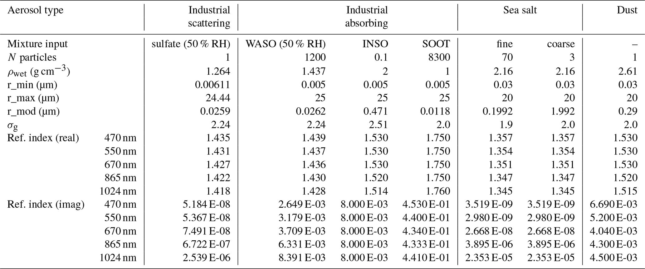
2.2 Aerosol types
Four aerosol types have been defined. Aerosol size distributions are assumed to be log-normal with the parameters shown in Table 1. Refractive indices are taken from the literature (see Table 1) and the aerosols are assumed to be internally mixed, with a volume-weighting rule. The four aerosol types defined in this benchmark have been chosen to represent a variety of size and optical properties observed in the atmosphere. Two fine-mode aerosols are defined: industrial scattering (aer_is) is sulfate aerosol with a relative humidity of 50 %, while industrial absorbing (aer_ia) is a mixture of the Optical Properties of Aerosols and Clouds (OPAC; Hess et al., 1998) aerosol type INSO (insoluble), SOOT (soot), and WASO (water soluble, at 50 % of relative humidity). The industrial absorbing aerosol is similar to an organic-matter aerosol type. We also consider a monomodal dust aerosol and a bimodal sea salt aerosol (aer_ss).
Table 1Aerosol physical and optical properties for the different aerosol types considered in the benchmark. σg is the geometric standard deviation. The refractive indices are linearly interpolated from the OPAC database (Hess et al., 1998). Dust refractive indices are linearly interpolated from Woodward (2001).
2.3 Aerosol optical properties
Aerosol optical properties were computed by the authors using their own Mie routines, and results were cross-checked for consistency. The Mie routine used to generate the input data was rewritten in Fortran based on the implementation of Toon and Ackerman (1981) and was compiled with the Intel Fortran compiler in quadruple precision. The calculations are monochromatic (i.e. no integration was performed on the wavelength). The aerosol size distribution is integrated over the size range reported for each type in Table 1, with a Gaussian quadrature of 10 000 points in logarithm of the radius. The number of terms used to compute the sums of the an and bn coefficients is approximated as a function of the Mie parameter () following Wiscombe (1980).
For each aerosol type, we provide the aerosol optical depths at the 440, 670, 865, and 1024 nm wavelengths corresponding to the selected AOD at 550 nm. The aerosol mass extinction coefficient (although not necessary to conduct the RTM calculations), single-scattering albedo, and asymmetry parameter are also given.
The phase matrix is computed and provided at 50 000 points evenly spaced in scattering angle from 0 to 180∘. As the particles are assumed to be spherical, only the S11, S12, S33, and S34 elements of the phase matrix are non-zero and provided. We also decompose the phase matrix in generalized spherical functions (de Rooij and van der Stap, 1984; de Haan et al., 1987) as needed for the vector version of the discrete ordinate method. For this, the phase matrix is integrated with an 8000-point Gaussian quadrature over the cosine of the scattering angle, and we provide the first 750 moments of that decomposition for the six commonly used elements (α1, α2, α3, α4, β1, β2). For completeness, we also provide the corresponding Legendre coefficients (by definition, the lth Legendre coefficient equals the lth Legendre moment multiplied by 2l+1). Thus, we provide all necessary information on aerosol optical properties for the usual RTMs so that no further processing of the aerosol optical properties should be required. Of course, the RTMs that neglect polarization should only consider the S11 term of the phase matrix or the α1 Legendre moments.
The accurate reconstruction of the original phase function from the Legendre decomposition (S11) cannot be ensured when a low number of Legendre moments is used to approximate it. As for the vertical resolution, there is no obligation for this benchmarking exercise to represent the exact phase function, and it may be interesting to approximate it to strike a balance between accuracy and computational cost (see, for example, Ding et al., 2009). The minimum number of Legendre moments for which the approximated phase function is positive depends on the aerosol type and the wavelength (basically, on how large the forward peak is). For the industrial scattering and industrial absorbing aerosols, a minimum of four to eight moments is required (depending on the wavelength). For dust aerosol, the minimum is between 14 moments (at 1024 nm) and 40 moments (at 470 nm), while for sea salt, the minimum is between 144 moments (at 1024 nm) and 348 moments (at 470 nm).
Figure 1 shows the phase function and the linear depolarization ratio for the four aerosol types considered in this benchmark.
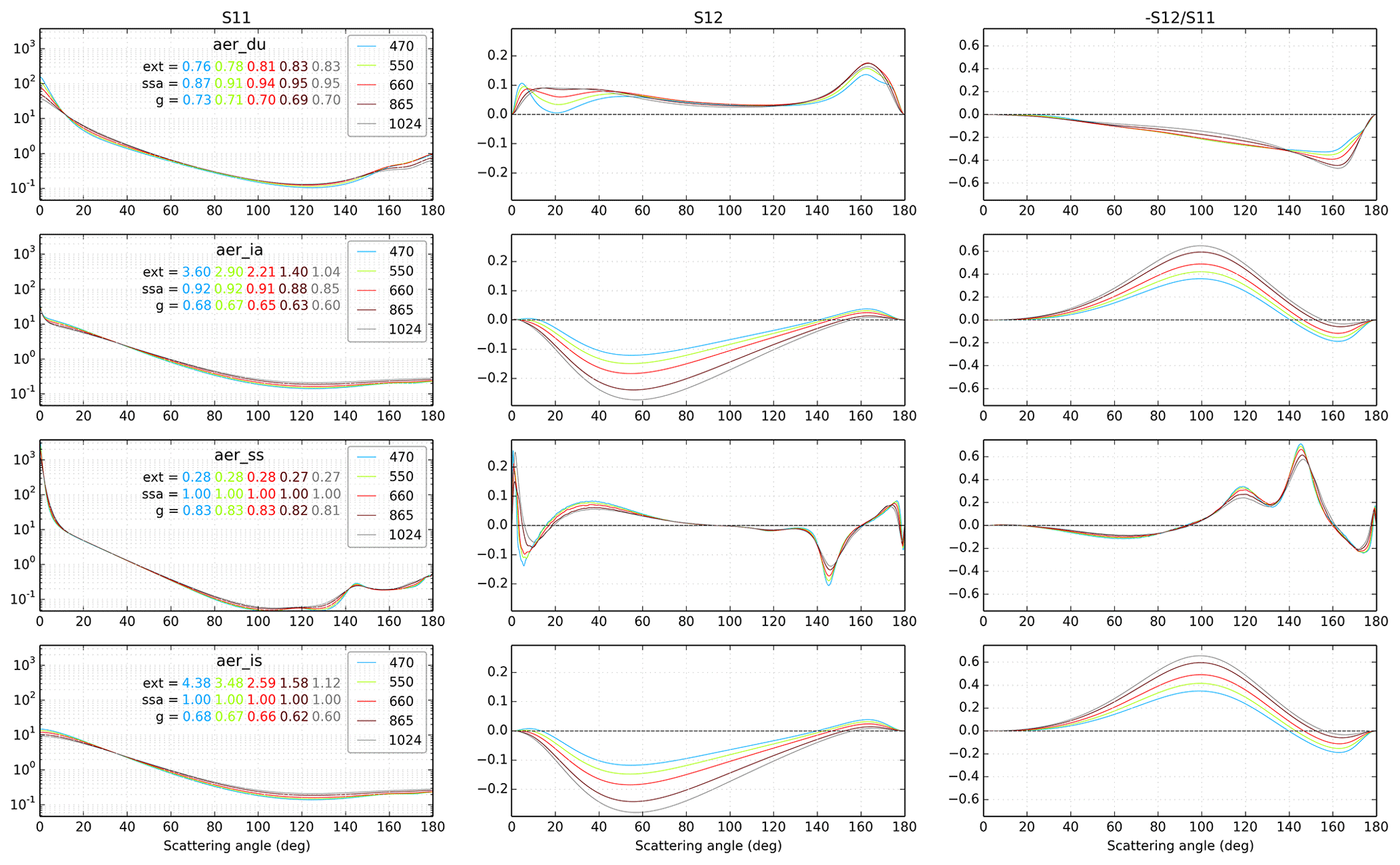
Figure 1First (i.e. S11, left panels) and second (i.e. S12, middle panels) element of the phase matrix and linear depolarization ratio (i.e. ) (right panels) as a function of the scattering angle (∘) for the four aerosol types (rows), where aer_du stands for dust, aer_ia for industrial absorbing, aer_ss for sea salt, and aer_is for industrial scattering. The colour code corresponds to the five wavelengths (470, 550, 660, 865, and 1024 nm). The mass extinction coefficient (ext, in m2 g−1), single-scattering albedo (ssa), and asymmetry parameter (g) are also indicated in each panel. The phase function is normalized to 2 .
2.4 Surface reflectance
Two surface reflectance models are selected: a Lambertian and an oceanic bidirectional reflectance distribution function (BRDF) model. For the Lambertian model, three surface albedos were chosen, namely 0, 0.05, and 0.1. The spectral dependence of the surface reflectance is ignored; i.e. the albedo is assumed to be the same for the five wavelengths considered. The second surface reflectance model is the oceanic glitter model from Mishchenko and Travis (1997). This model is suited for both full vector radiative transfer models (i.e. including polarization) and for the scalar approximations.
Wind speed is set to 10 m s−1, but the Mishchenko and Travis (1997) code assumes an isotropic Gaussian distribution of (oceanic) surface slopes, so the wind orientation is not taken into account. The salinity is set to 34.3 ‰ and water refractive indices are interpolated, for each wavelength, from the data provided in Hale and Querry (1973) as inputs to the Mishchenko and Travis (1997) routine (available at https://www.giss.nasa.gov/staff/mmishchenko/brf/, last access: 19 February 2019). The effect of shadowing is also taken into account.
The convention for the azimuthal angle used in the Mishchenko and Travis (1997) routine is the opposite of the convention that we use below to define geometries, so the coupling between the atmospheric RTM and the oceanic code has to be done carefully.
2.5 Geometries and configurations
We have selected eight cases for aerosol loadings in the atmosphere, with AOD at 550 nm ranging between 0 (no aerosol) and 2 (high aerosol loading). These values refer to the 550 nm wavelength, and the corresponding AODs can be estimated for the other wavelengths depending on the aerosol types. A table with the equivalences in AOD for each aerosol type and wavelength is also provided in the benchmark protocol.
We have further selected four solar and four viewing zenith angles – θs and θv – from 0∘ (zenith) up to 60∘. Given the provided surface reflectance models and the assumption of spherical (hence randomly oriented) aerosols in the atmosphere, the radiance at the top of the atmosphere is only dependent on the difference between the incident and reflected azimuthal angle and not on each value taken independently. We have chosen five azimuthal angles between ϕr=0∘ (backscatter when solar and viewing zenith angles are equal) and ϕr=180∘ (forward scattering when solar and viewing zenith angles are equal). The different cases are summarized in Table 2. Removing the redundancies in aerosol types for AOD =0 and azimuthal angle for , this results in 11 020 cases for the BRDF surface and 33 060 cases for the Lambertian surfaces (see Table 3), which gives a grand total of 44 080 cases.
Table 2Summary of the proposed geometrical and environmental conditions used in the simulations.
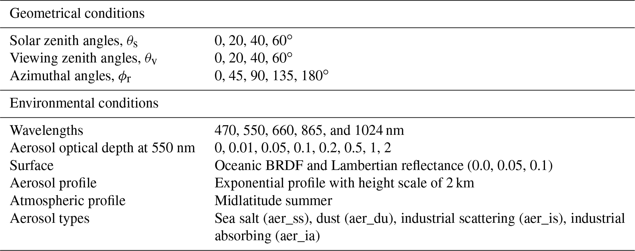
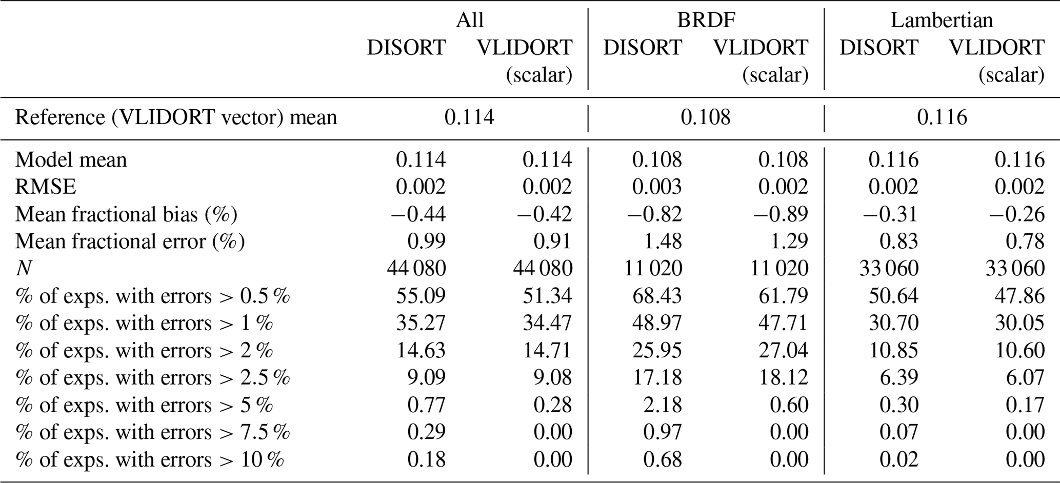
Table 3Statistical measures of DISORT and scalar VLIDORT reflectances against vector VLIDORT (first row). Errors of the last rows are defined as the absolute value of the relative error, using the VLIDORT (vector) reflectance as the reference. VLIDORT is the configuration with 32 streams and the TMS correction activated. N refers to the number of cases.
2.6 Measured variables
We aim to provide a standardized dataset to evaluate the possibility of assimilating satellite radiances in operational forecasts of atmospheric composition. Thus, two variables are important to estimate for each case: the simulated reflectance (or radiance) that would be observed by the satellite and a “sound” estimate of the radiative transfer code runtime.
We will describe the accuracy of the models in terms of the reflectance, ρI, of the intensity (i.e. the first Stoke component), which is related to the radiance, I, through the following relationship:
where Is is the incident solar flux at the top of the atmosphere (conveniently taken to equal 1 for reflectance calculations) and θs is the solar zenith angle.
The runtime may be difficult to estimate and compare between different models. We aim to measure the runtime of the computations excluding input/output operations, as typical applications would embed the RTM code in a larger operational system. The runtime of the RTM should be measured in a single-thread configuration. Ideally, the simulations should be performed on the same core of the computer and with the same system load conditions (except for the RTM) as other threads on the operating system (in particular with a high input/output load) could hamper the correct timing of the model. Multiple repetitions of the computations can be performed to get better estimates.
Given a set of atmospheric and aerosol conditions, some models can compute, almost without extra cost, the radiances for several viewing geometries, while other models require multiple simulations to achieve the same. For this protocol, this would introduce a difference of a factor of circa 80 (the number of viewing geometries) in the reported runtimes. Depending on the application, this feature of some models may or may not be relevant. For this reason, we present here the runtimes of the tested models in two configurations: one taking advantage of the simultaneous output for multiple viewing geometries and another one without this feature. In the second configuration (called “ind” in Sect. 3), each simulation outputs only one geometry while in the first configuration (called “mult” in Sect. 3), it outputs as many values as possible within the specifications of the protocol. The number of multiple outputs per simulation will be detailed in the next section.
3.1 Reference model: VLIDORT
The VLIDORT model is an independent implementation of the discrete ordinate method based in part on earlier work by Siewert (2000a, b) and other sources. In this work we used the VLIDORT version 2.7, which includes a BRDF supplement that can be called before the main program. A detailed user's guide is available (Spurr, 2014). One interesting feature of this model is that it also provides Jacobians with respect to the model inputs (not used in this study). In this model, it is possible to choose how many elements are computed in the Stokes vector. Although VLIDORT is able to solve the radiative transfer equation for the four-element Stokes vector (Spurr, 2008), we will refer to the vector runs when the 3×3 approximation of the RT problem is used (i.e. neglecting circular polarization in the atmosphere by solving only for ) and we will refer to the scalar runs when only the first element of the Stokes vector is used in the computations (i.e. when polarization of electromagnetic radiation is not accounted for). VLIDORT is written in double precision; it has the capability to output, in a single call, radiances for any number of solar and viewing angles. The protocol vertical resolution with 49 layers is used. It should be noted that the discrete ordinate method shows a numerical instability for zenith viewing angle θv of 0∘ or a relative azimuthal angle ϕr of 90∘. These angles are therefore prescribed at θv=0.0001∘ and ϕr=89.98∘ instead to circumvent this problem. We use the model with 32 streams, and the TMS correction (Nakajima and Tanaka, 1988) is activated. The TMS correction removes the single-scattering feature computed with a few streams and replaces it by the exact single-scattering contribution. This correction helps to remove non-physical features due to the use of a low number of Legendre coefficients in the computation. The VLIDORT vector is our reference model.
3.2 DISORT
The DISORT model (Stamnes et al., 1988) is a flexible and widely used RTM. It solves the scalar approximation of the radiative transfer equation in a plane-parallel atmosphere by using the discrete ordinate method. In this study, we use the DISORT code, version 4, available from http://lllab.phy.stevens.edu/disort/ (last access: 19 February 2019), and we coupled the oceanic BRDF following the code developer instructions. We use the model with 32 streams, and the TMS correction (Nakajima and Tanaka, 1988) is activated. It should be noted that most of this code is written in single precision, but important routines (such as the computation of the Gaussian nodes) are written in double precision. We use 32 streams in our main configuration, but sensitivity results for 4, 8, 16, 32, 64, 96, and 128 streams are also presented below. The protocol vertical resolution with 49 layers is used. Similar to VLIDORT, the DISORT code has numerical instabilities which manifest themselves when the solar and viewing zenith angles (θs and θv) are equal. In such cases, we perturb the cosine of the viewing zenith angle by .
Given a solar zenith angle, the DISORT model can provide outputs for multiple viewing geometries. In this study, the number of geometries for the mult timing configuration is the number of ϕr cases multiplied by the number of θv cases (i.e. ).
Although we know the DISORT model to be too slow for online data assimilation of aerosol radiances, we find it useful to document here the trade-off between accuracy and computing time as a function of the number of streams used in the calculations. Figure 2 shows both the mean fractional error and the average computing time for 4, 8, 16, 32, 64, 96, and 128 streams. The mean fractional error is shown relative to our reference VLIDORT (vector) and is of the order of 1 or 1.5 % for the Lambertian and oceanic BRDF surface cases, respectively, as soon as the number of streams exceeds eight. Most of that discrepancy is because DISORT neglects the polarization. When DISORT is compared to VLIDORT (scalar), the mean fractional error is significantly smaller: <0.1 % for the Lambertian surface case and <1 % for the surface BRDF case.
There is a big gain in accuracy when increasing the number of streams from 4 to 8 and little further gain in accuracy beyond 16 streams. A deterioration in accuracy is observed beyond 96 streams in the case of the BRDF surface, which may be due to the DISORT model being coded in single-precision float. While the dependence of model accuracy on the number of streams is well known (Stamnes and Swanson, 1981), we find it useful to confront the loss of accuracy with the gain in computational cost. Computing time increases rapidly with the number of streams (faster than the cube of the number of streams beyond 16 streams). Using 16 streams might, therefore, be an interesting trade-off between accuracy and computational cost.
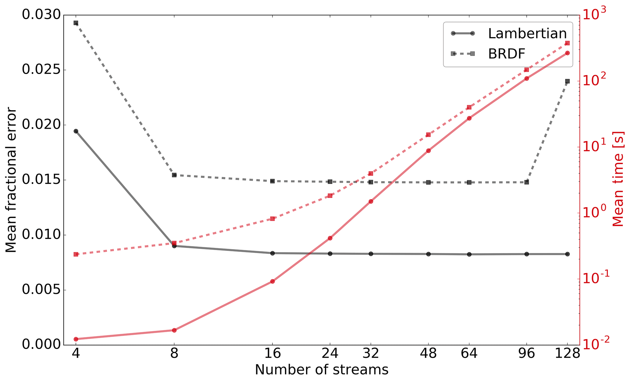
Figure 2Accuracy (in black) and computing times (in red) for the DISORT model as a function of the number of streams used. The Lambertian and oceanic BRDF surface cases are shown with solid and dashed lines, respectively. The accuracy is shown in terms of mean fractional error against VLIDORT (vector). The computing times are an average for 20 geometries and were estimated on a processor AMD Opteron 6378, 2.4 GHz. Please note the logarithmic scales for the number of streams used in the DISORT calculations (x axis) and the timings (right vertical axis).
3.3 6SV2
The 6SV2 model is a radiative transfer model based on the successive order of scattering (SOS) method (Vermote et al., 1997). It solves the radiative transfer equation by using the three-element approximation (3×3) of the Stokes vector. The accuracy of the code against previous benchmark and Monte Carlo codes has been reported to be better than 1 % (Kotchenova et al., 2006; Kotchenova and Vermote, 2007). We have used version 2.1 of the model. Two configurations are available: a standard accuracy configuration that consists of 83 Gaussian points for the phase function, 30 vertical levels, 25 zenith angles, and 181 azimuth angles and a high-accuracy configuration that consists of 121 Gaussian points for the phase function, 50 vertical levels, 75 zenith angles, and 181 azimuth angles. We will present results only from the standard accuracy, which is 2 to 70 faster than the high-accuracy configuration, but will comment briefly on the high-accuracy configuration in Sect. 4.2.
Molecular scattering and absorption vertical profiles are embedded in the code. Both are internally computed according to the atmospheric profile as part of “core” SOS routines. It is therefore not appropriate to prescribe our own molecular scattering and absorption profiles, so we use the 6SV2 defaults instead. The difference in the total molecular scattering optical depth is less than 0.26 % with respect to the files provided in this protocol. We have coupled the BRDF calculations to the 6SV2 model, but it should be noted that the atmosphere–surface coupling of the oceanic BRDF model in 6SV2 does not use the full surface reflection matrix but only the first column of it (i.e. the column that relates reflected I with incoming I, Q, and U).
The 6SV2 model can only compute one viewing geometry in each model call (i.e. the ind configuration is exactly the same as the mult configuration).
3.4 FLOTSAM
We also test in this study a preliminary version of the Forward-Lobe Two-Stream Radiance Model (FLOTSAM), which is being developed at the European Centre for Medium-Range Weather Forecasts (ECMWF). Unlike a lookup-table-based solar RTM, FLOTSAM permits an arbitrary layering of different types of scatterers, including clouds, aerosols, and molecules. The model has been designed to be fast enough to be used in iterative assimilation and retrieval schemes. It exploits the fact that particle phase functions typically contain a “narrow forward lobe” associated with scattering angles of less than a few degrees and a “wide forward lobe” associated with scattering angles of the order of 15∘. This enables coupled ordinary differential equations to be written down for radiation in the quasi-direct solar beam (including the narrow forward lobe) and a wider beam of radiation propagating away from the Sun due to scattering by the wide forward lobe. Additionally, the upwelling and downwelling diffuse fluxes are computed using the two-stream approximation. FLOTSAM may, therefore, be thought of as the solar analogue of the infrared two-stream source function technique of Toon et al. (1989). To facilitate the use of FLOTSAM in variational assimilation and retrieval schemes, it has been coded in C++ using version 2.0 of the Adept library (Hogan, 2014, 2017), which enables the Jacobian to be easily computed via Adept's fast automatic differentiation capability. FLOTSAM has been incorporated into the Cloud, Aerosol and Precipitation from Multiple Instruments using a Variational Technique (CAPTIVATE) retrieval scheme, which will provide operational products from the forthcoming EarthCARE satellite (Illingworth et al., 2015).
FLOTSAM is designed to be used in iterative schemes in which multiple calculations are performed with different profiles of optical properties but for the same viewing geometry. This is implemented by allowing the user to perform the set-up calculations once for a particular solar zenith angle, viewing zenith angle, and viewing azimuth angle and then to reuse the information in subsequent radiance calculations for different optical profiles. We assess the computational cost for both the ind and the mult configurations, with the latter consisting of cases involving 80 geometry set-up calculations and each separate geometry being used with eight different optical depths.
4.1 Methods and statistics
The protocol has been tested for the five model versions described above: VLIDORT (vector), VLIDORT (scalar), DISORT, 6SV2, and FLOTSAM. As explained in Sect. 2.6, the accuracy is quantified in terms of monochromatic reflectances at the top of the atmosphere and the accuracy is computed against the vector version of the VLIDORT model unless stated otherwise.
With as many as 44 080 cases considered in this study, we have to find original ways to visualize the results as explained below. Along with the average reflectance computed for each model, the following statistical measures have also been computed:
where N is the number of experiments, mi is the reflectance of the tested model, and ri is the reflectance of the reference model for case i. By definition, the mean fractional bias can range between −2 and 2, with a best score of zero, while the mean fractional errors can range between 0 and 2, with a best score of zero. Both values are multiplied by 100 with respect to the definitions above in the tables presented below. We also state the percentages of cases where the relative error of the reflectances is above defined relative error thresholds. These diagnostics, which could be detailed for particular subsets of our 44 080 cases, can help to decide if and under which conditions a particular RTM could be useful, according to the required accuracy of the reflectance calculations.
Runtimes of the models are presented in an absolute measure (seconds), and no reference is needed. Finally, we will comment on possible trade-offs between accuracy and computing time.
4.2 Accuracy
Figure 3 shows histograms of the simulated reflectances of the VLIDORT (vector) model at the top of the atmosphere for all or various subsets of the 44 080 cases. These reflectances form the reference simulations for this study. The width of the histograms (or violins) in Fig. 3 is proportional to the number of cases in each bin of the reflectance (y axis) discretization. The multiple panels (and multiple violins) are computed with all the simulations but filtered by the value indicated on the x axis. Therefore, they can be interpreted as analogous to marginal density probability functions of the set of simulations. Figure 3 shows a wide range of reflectances (from near 0 to almost 0.5) and known dependencies of the reflectance with respect to some of the input variables such as the surface albedo (Lambertian case), the AOD, or the wavelength in this range of the spectrum.
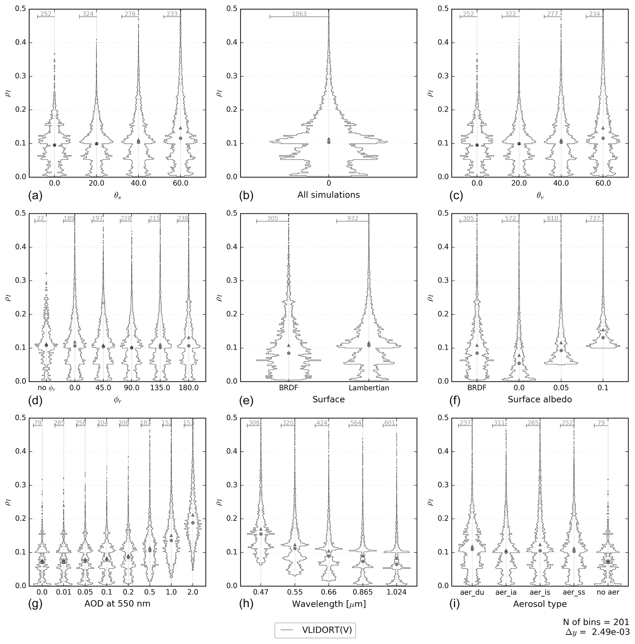
Figure 3Histograms of the computed reflectances for the VLIDORT model. Panel (b) is a histogram of all considered cases, while the other panels classify the cases according to the value of θs (a), θv (c), (d, “no ϕr” corresponds to the cases where ), and surface type – BRDF or Lambertian (e), surface albedo value (f), 550 nm aerosol optical depth (g), wavelength (in µm, h), and aerosol type (“no aer” corresponds to AOD =0, i). The width of the classes is indicated at the bottom right (), and the maximum number of cases in a class is provided for each histogram. The histograms are presented as “violin plots” with a rotated density plot on each side. Mean (triangles) and median (circles) values are indicated. Note that the scale used on the x axis is different for each violin plot.
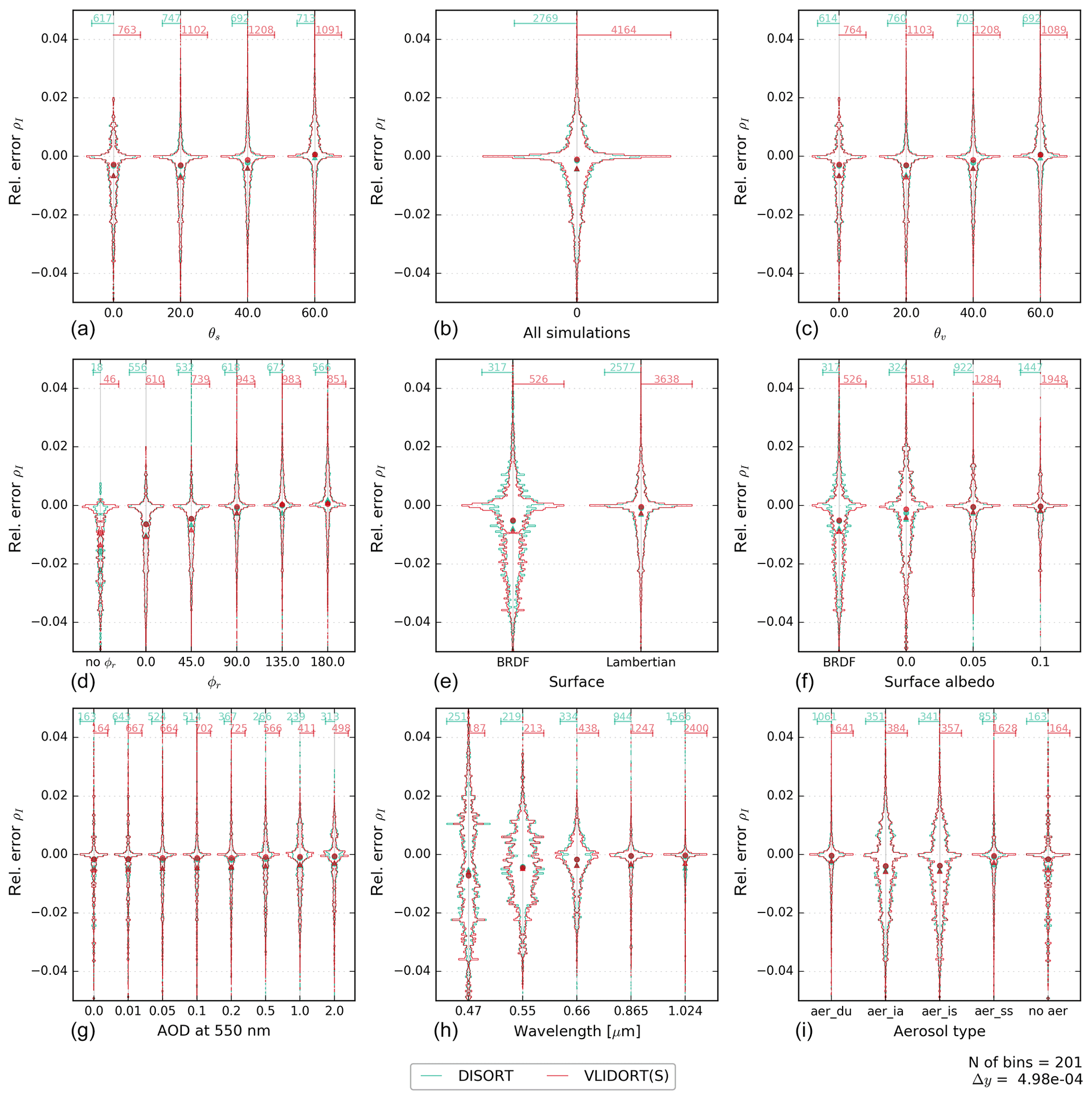
Figure 4Same as Fig. 3 but for the relative error of the DISORT and VLIDORT (scalar) models against the vector version of VLIDORT. Please note the ±5 % error range on the y axis. The number of cases outside the range is indicated in Table 3. The width of the classes is . Note that the scale used on the x axis is different for each violin plot but is the same for the two models within a violin plot.
A first comparison of the relative error is shown in Fig. 4 for two scalar models (with otherwise the same degree of sophistication as the reference model). Figure 4 shows the histograms of the relative errors, , with m being the tested model and r the reference model (the vector version of VLIDORT). It can be seen that for both models, DISORT and the scalar version of VLIDORT, the errors are mostly below 5 %. They are centred on zero for the Lambertian surface, but a negative bias is observed for the BRDF case. Comparison of scalar VLIDORT against vector VLIDORT provides a direct measure of the relative errors due to neglecting polarization in the model. As expected and because of a larger molecular scattering contribution, we observe larger relative errors for the shorter wavelengths (MFE =1.8 % at 470 nm; MFE =0.5 % at 1024 nm). We also observe larger errors for the accumulation-mode aerosols (industrial scattering and industrial absorption have MFE ≈1.2 %) in contrast to coarse-mode aerosols (dust and sea salt have MFE ≈0.6 %). These errors are associated with the larger polarized phase function (see Fig. 1) of industrial scattering and industrial absorption aerosols for large AOD (see Figs. A2 and A4). Although no clear relation is shown for relative errors as a function of the geometrical parameters in Fig. 4, Fig. A2 shows a clear link between the relative errors and the scattering angle for these two accumulation-mode aerosols at large AOD. The oceanic BRDF function used in this study also enhances the errors of the scalar versions as these neglect the polarizing effect of the surface because the glint can increase the polarized feature of the light for some angles. Larger relative errors are shown for the dark surface case (Lambertian surface albedo equal to zero has MFE ≈1.2 %) because the reference reflectances are smaller than for their 0.05 and 0.1 Lambertian counterparts (with MFE ≈0.7 % and MFE ≈0.5 %, respectively). The error statistics of the VLIDORT (scalar) and DISORT models are very similar, with noticeable differences only for the BRDF case (Fig. 4 and Table 3). The scalar approximation may thus be appropriate for some combinations of wavelengths, aerosols types, and surface types but not for others. We further note, that for both types of surfaces, the scalar VLIDORT simulations outperform DISORT simulations when they are compared against the vector version of VLIDORT (which is not surprising), but in both cases the overall mean fractional error is larger than 0.7 % and the mean fractional bias is negative.
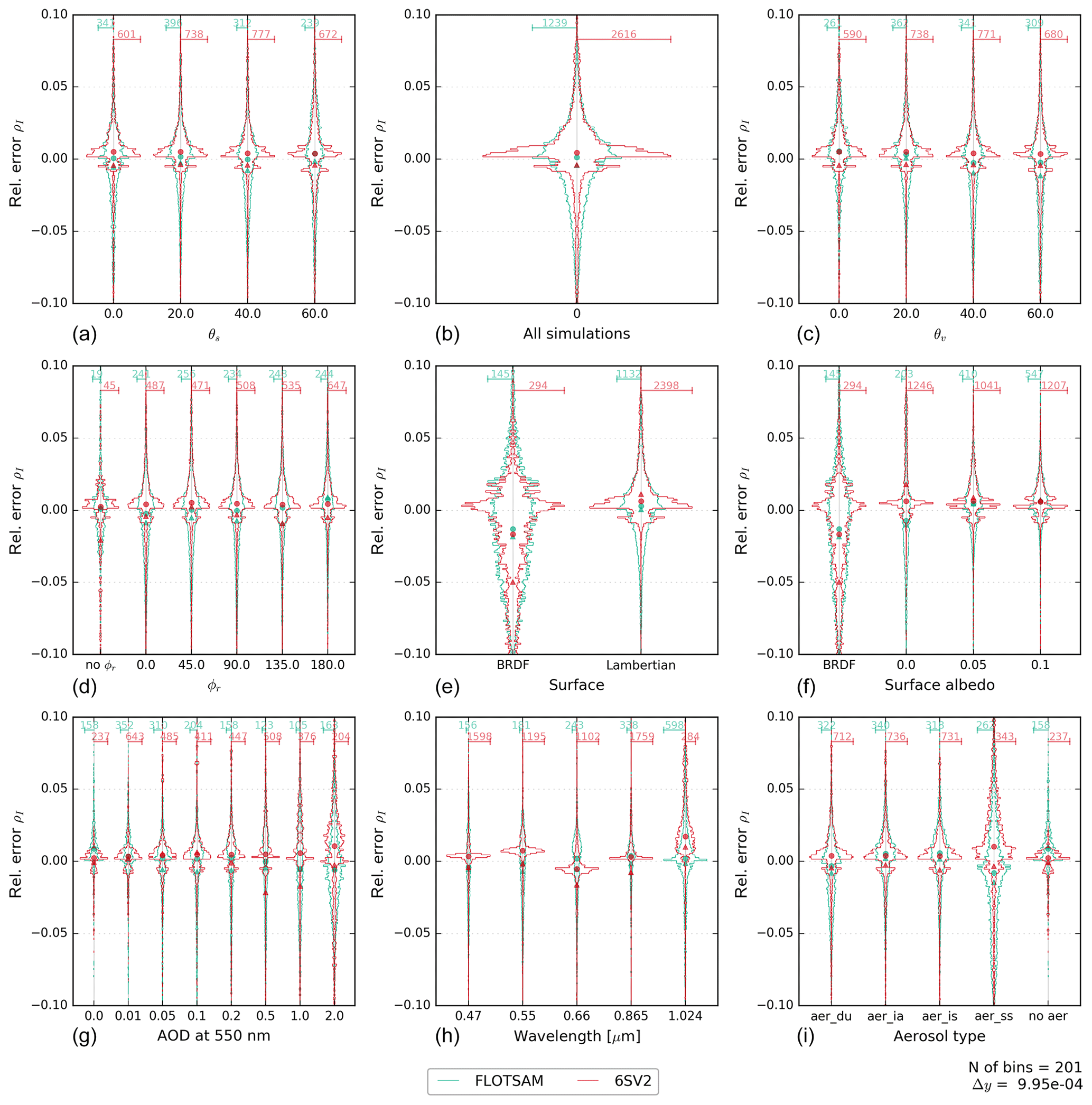
Figure 5Same as Fig. 3 but for the relative error of the FLOTSAM and 6SV2 models against the vector version of VLIDORT. Please note the ±10 % relative error range of the y axis. The width of the classes is . The number of cases outside the range is indicated in Table 4. Note that the scale used on the x axis is different for each violin plot but is the same for the two models within a violin plot.
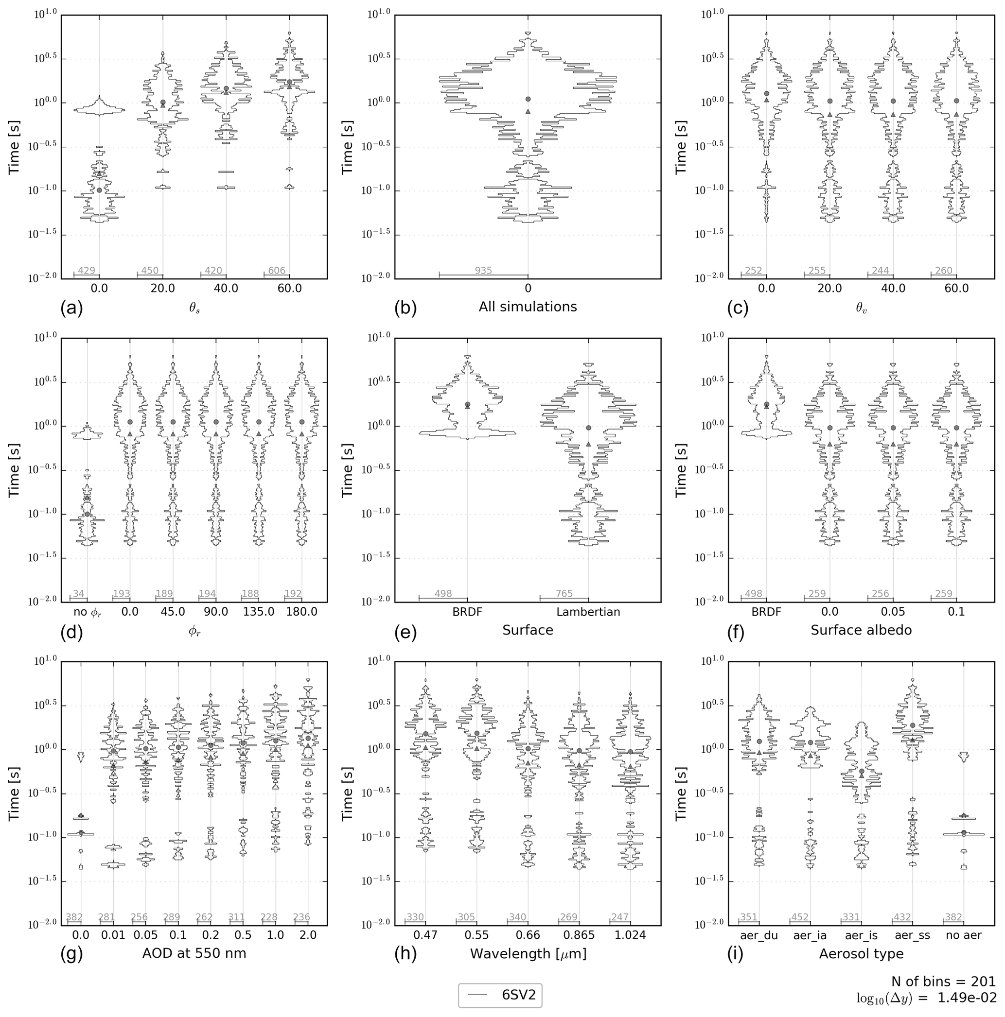
Figure 6Same as Fig. 3 but for the runtime of the 6SV2 model. Please note the logarithmic scale on the y axis.
Figure 5 and Table 4 show the relative errors of the other two models used in this study, 6SV2 and FLOTSAM, against VLIDORT (vector). As the FLOTSAM model does not include polarization, it is not expected to outperform the scalar approximations exemplified in the DISORT and VLIDORT (scalar) comparisons. However, this is the case for the 470 nm cases, as can be seen from the corresponding violin plot of Fig. 5. For 6SV2, the relative error shows a mode around zero, while for FLOTSAM, the shapes of the violin plots are more similar to those of the scalar approximations shown in Fig. 4. The reason for the unexpected dependence of the 6SV2 model errors on the wavelength is not completely clear, but it could be related to the technical difficulties in prescribing user-specific molecular scattering and absorption profiles in the 6SV2 code (see Sects. 2.1.1 and 3.3). In contrast to Fig. 4, Fig. 5 shows larger relative errors for sea salt aerosols for both models. While larger errors in Fig. 4 were related to the polarization/depolarization effects from aerosol particles (as shown in the right column of Fig. 1), errors of 6SV2 and FLOTSAM could be related to the more pronounced forward-scattering peak of the sea salt aerosols and their large single-scattering albedo. In fact, errors for large AOD (Fig. A3) are not strongly linked to the amount of polarized radiance (Fig. A4) for sea salt aerosols. In the case of 6SV2, the coarse discretization of the aerosol phase function used in the model configuration (83 Gaussian points, Sect. 3.3) hampers the accurate simulation of the sea salt forward-scattering peak. There is no clear dependence of the relative errors on the viewing and solar geometries but, as for Fig. 4, larger errors are observed for larger AOD and for the surface BRDF case.
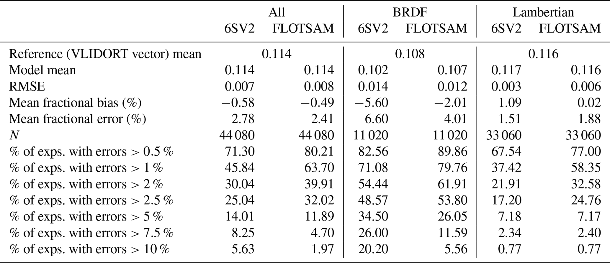
Synthetic error statistics are shown in Table 4. Both the 6SV2 and FLOTSAM models have comparable mean fractional errors, but these are larger than those of DISORT and VLIDORT (scalar). Some difference concerning the type of surface can be appreciated, with 6SV2 performing better in the case of Lambertian surfaces. It should be noted that using the high-accuracy configuration of 6SV2 instead of the standard accuracy configuration reduces the mean fractional error from 1.5 % to 1.1 % for the Lambertian surface case but does not improve this score for the BRDF surface case. The mean fractional bias is negative, and it is of similar magnitude for both models. However, 6SV2 presents larger biases over the two types of surfaces (and the sign of the bias differs for the BRDF and Lambertian surfaces). In contrast, FLOTSAM shows virtually no bias for the Lambertian surface cases and a smaller bias than 6SV2 for the BRDF cases. An important difference with the scalar models is the presence of a heavy tail in the relative error distribution, which can be inferred from the last rows of Table 4.
4.3 Timing
In this section, we present statistics of computing times for three of the models used in this study. All the computing times presented below were estimated on an Intel i5-4690, 3.5 GHz workstation running Linux (kernel 2.6.32), GNU C++ and Fortran compiler version 4.4.7, on a single processor and with exclusive use of the workstation. We have compiled the models using their default compilation flags, i.e. “-O” for 6SV2, “-O3” and “-march=native” for FLOTSAM, and “-O3” for DISORT.
We start this section with the 6SV2 model which can only be used in ind configuration. Figure 6 shows the violin plots of the computing time of the 6SV2 model that spans as much as 2 orders of magnitude. Clearly, the BRDF cases are more expensive than the Lambertian surface cases, with most computing times ranging between ca. 0.7 and 4 s for the former. This appears to be due to multiple calls to the BRDF routine. It may be possible to optimize this routine or recode it in a more efficient way, but we have not attempted to do so. We also note an increase in computing time with increasing solar zenith angle (θs) and AOD and with decreasing wavelength. This is consistent with a larger number of scattering orders being necessary in such cases. Cases for coarse mode aerosols (especially sea salt aerosols) are more expensive than cases for accumulation-mode aerosols, with some calculations reaching 5 s for sea salt aerosols. We do not have an explanation as to why the cases for industrial absorbing aerosols are more expensive than those for industrial scattering aerosols.
Table 5Average runtimes in seconds. The standard deviation is shown in parentheses. The mult runtimes account for 640 profiles for FLOTSAM, 20 profiles for DISORT, and 1 profile per model call for 6SV2. The one-off set-up costs of FLOTSAM are invoked only once per instance of the executable, no matter how many radiances are subsequently calculated, so are the same for the ind and mult experiments.
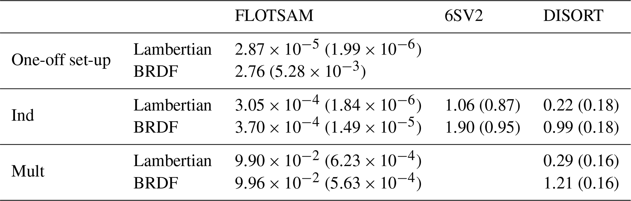
As discussed above, the DISORT and FLOTSAM models offer efficiency savings when multiple profiles are computed together. In the case of DISORT, multiple viewing geometries can be computed for one solar zenith angle. In the case of FLOTSAM, a smaller saving is that the geometry set-up calculations may be computed once for a given solar/viewing geometry and then reused for multiple atmospheric profiles with different optical properties. The runtime of these models is, in general, not sensitive to the viewing geometry, wavelength, aerosol type, or AOD. However, there are some differences between the two types of surface reflectance. Table 5 shows a summary of the measured runtimes for the three tested models. Computing times are indicated for the two measurement procedures (ind and mult) and for the two types of surface reflectance (BRDF and Lambertian). In the case of FLOTSAM, we also report the “one-off set-up” cost, which in the case of the BRDF involves creating a four-dimensional lookup table. We stress that this is invoked only once per call to the executable, so in an operational data assimilation system performing many millions of radiance calculations it would increase the executable runtime by only a very small fraction. The one-off set-up costs are not shown for the 6SV2 and DISORT models as they are not isolated from the rest of the computations.
For the 6SV2 model, values of Table 5 are in concordance with Fig. 6 with runtimes of the order of seconds. The DISORT model average runtime is smaller than that of 6SV2. Similarly to 6SV2, there is an important dependence of the DISORT runtime on the type of surface considered. The extra cost of computing 20 profiles, instead of 1 profile, can be estimated as the difference between the mult and ind cases. For DISORT, this additional cost is about 0.07 s for the Lambertian case and about 0.22 s for the BRDF case, which correspond to 25 % and 18 % of the total mult runtime. This would benefit an application that requires simultaneous calculation of many viewing geometries. The spread of DISORT runtimes indicated in Table 5 arises because DISORT efficiently decreases the number of internal computations for symmetric geometries (solar zenith angle equal to zero, 21 % of the cases), and it is faster for AOD =0 (3.4 % of the cases). For the remaining cases of Table 5, there is almost no spread in the DISORT runtime.
Table 5 shows the runtimes of the FLOTSAM model. Firstly, it is noted that the standard deviation of the reported values is small (around 1 order of magnitude less than the values). This is because FLOTSAM performs the same number of operations for every case; thus, there is no added value of showing histograms of runtimes. For this model, it can be seen that the one-off set-up cost of the BRDF is a little under 3 s, but in the ind case, subsequent radiance calculations are 3–4 orders of magnitude faster than the other two models tested, and the BRDF calculation is only slightly slower. If many profiles have to be computed with the same observation geometry, then the geometry set-up cost is invoked only once and the average cost per profile is reduced. This is illustrated in the mult case in which 640 profiles are computed, which involves 80 different geometries. Excluding the model set-up time, the computation of a single profile takes around 0.3 to 0.4 ms in the ind case and around ms in the mult case.
In this study, we have presented a comprehensive benchmarking methodology and protocol, with an unprecedented number of cases combining different viewing geometries, aerosol optical depths, aerosol types, wavelengths, and surface types. The VLIDORT model in its vector configuration (i.e. considering polarization) is used as the reference model. Preliminary results in terms of accuracy and computing time are presented for three models: the well-known models DISORT and 6SV2, on the one hand, and FLOTSAM, a new fast model under development by two of the authors of this study, on the other. All models perform better when using Lambertian surface reflectance than when using an oceanic BRDF. All the models perform better under low AOD, and the scalar models have lower accuracies at shorter wavelengths. For the Lambertian surface cases, the mean fractional errors of the models are 0.8 %, 1.5 %, and 1.9 % for DISORT, 6SV2, and FLOTSAM, respectively. The BRDF cases show a larger mean fractional error with 1.5 %, 6.6 %, and 4 % for DISORT, 6SV2, and FLOTSAM, respectively.
The DISORT and 6SV2 models show comparable computing time, between tenths of a second and seconds, but DISORT can provide the solution at multiple viewing geometries for each atmospheric condition, while 6SV2 cannot. FLOTSAM is very fast, with computing times of much less than 1 ms per profile. However, it should be noted that this model is still under development and its accuracy could improve further. Moreover, all models present a tail of cases with larger errors and/or computing times. It could be interesting to characterize these better to investigate if screening out those cases can be an option in data assimilation applications. Also, a fast tangent linear and adjoint computation is required for the integration of an RTM in a variational data assimilation system.
The protocol and input and output data are available as a potential resource for interested developers and users of RTMs willing to benchmark their models.
The detailed protocol is available in PDF format. All inputs necessary to the benchmark are available as ASCII text files. The surface BRDF is available as a Fortran routine from the Michael Mishchenko website https://www.giss.nasa.gov/staff/mmishchenko/brf/ (Mishchenko and Zakharova, 2019). The VLIDORT reference results are available in NetCDF format.
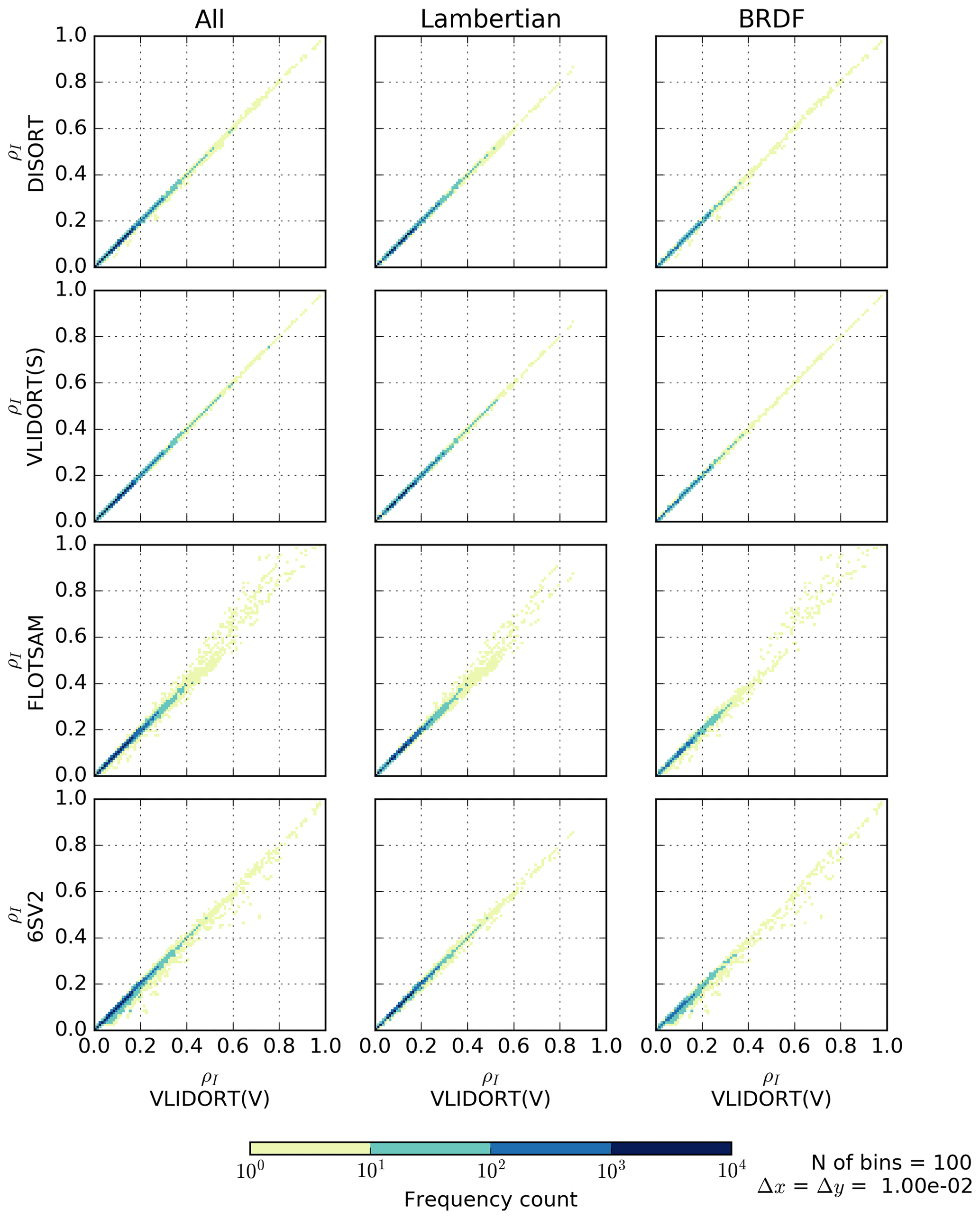
Figure A1Two-dimensional density plots of the simulated reflectances for the 6SV2, FLOTSAM, DISORT, and VLIDORT (scalar) models versus those of the VLIDORT (vector) model. The plots in the left column mix all 44 080 cases, while those in the middle and right columns are for the Lambertian and BRDF surface cases, respectively.
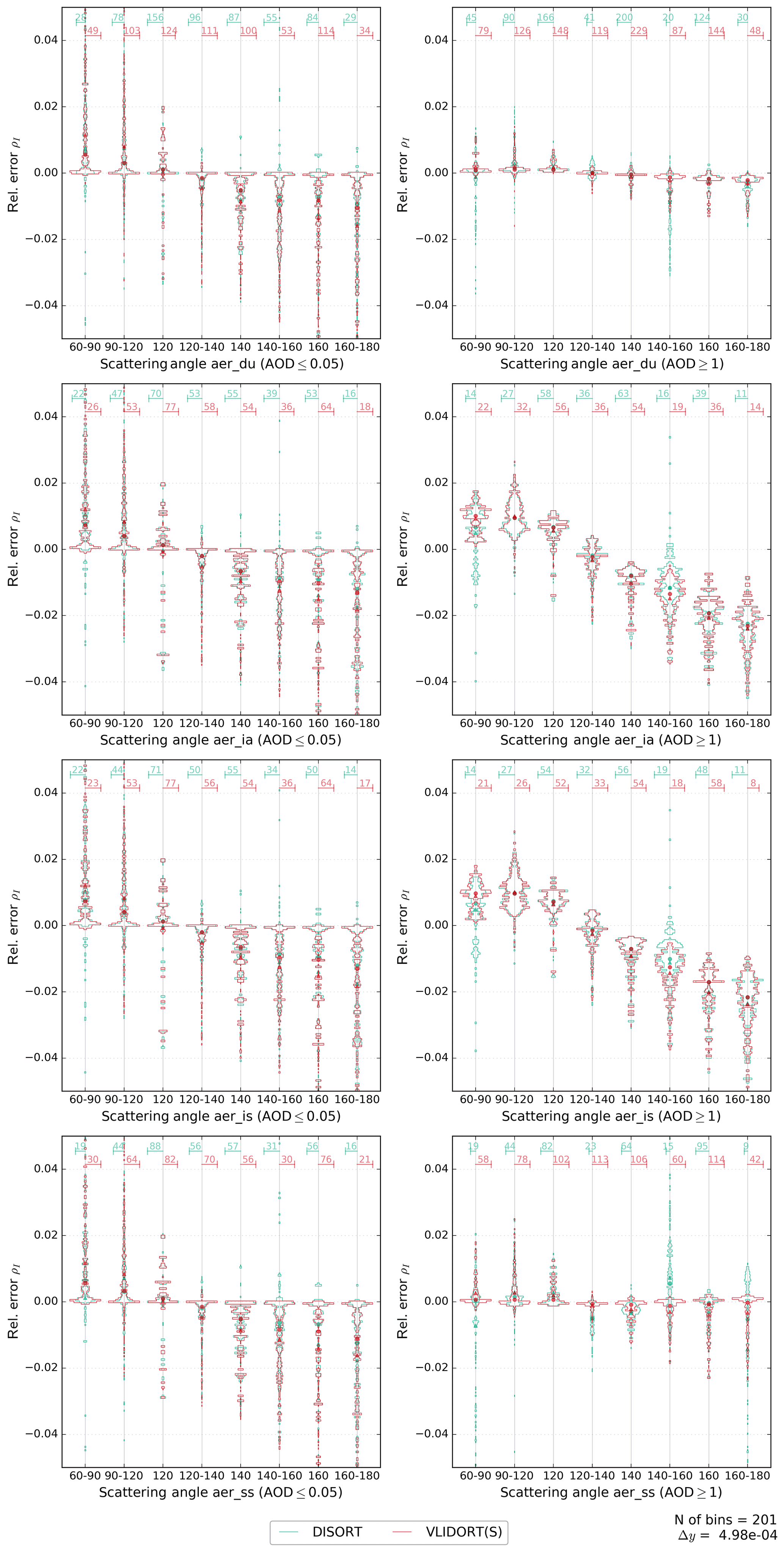
Figure A2Histograms for the relative error of the VLIDORT (scalar) and DISORT models. Similar to Fig. 4 but only for AOD ≤0.05 on the left column and AOD ≥1 in the right column (AOD at 550 nm). Relative error histograms are presented as a function of the scattering angle. The scattering angle has been binned at intervals with a similar quantity of data. The four aerosol types considered in this work are shown in different panels.

Figure A3Histograms for the relative error of the FLOTSAM and 6SV2 models. Similar to Fig. 4 but only for AOD ≤0.05 in the left column and AOD ≥1 in the right column (AOD at 550 nm). Relative error histograms are presented as a function of the scattering angle. The scattering angle has been binned at intervals with similar quantities of data points. The four aerosol types considered in this work are shown in different panels.
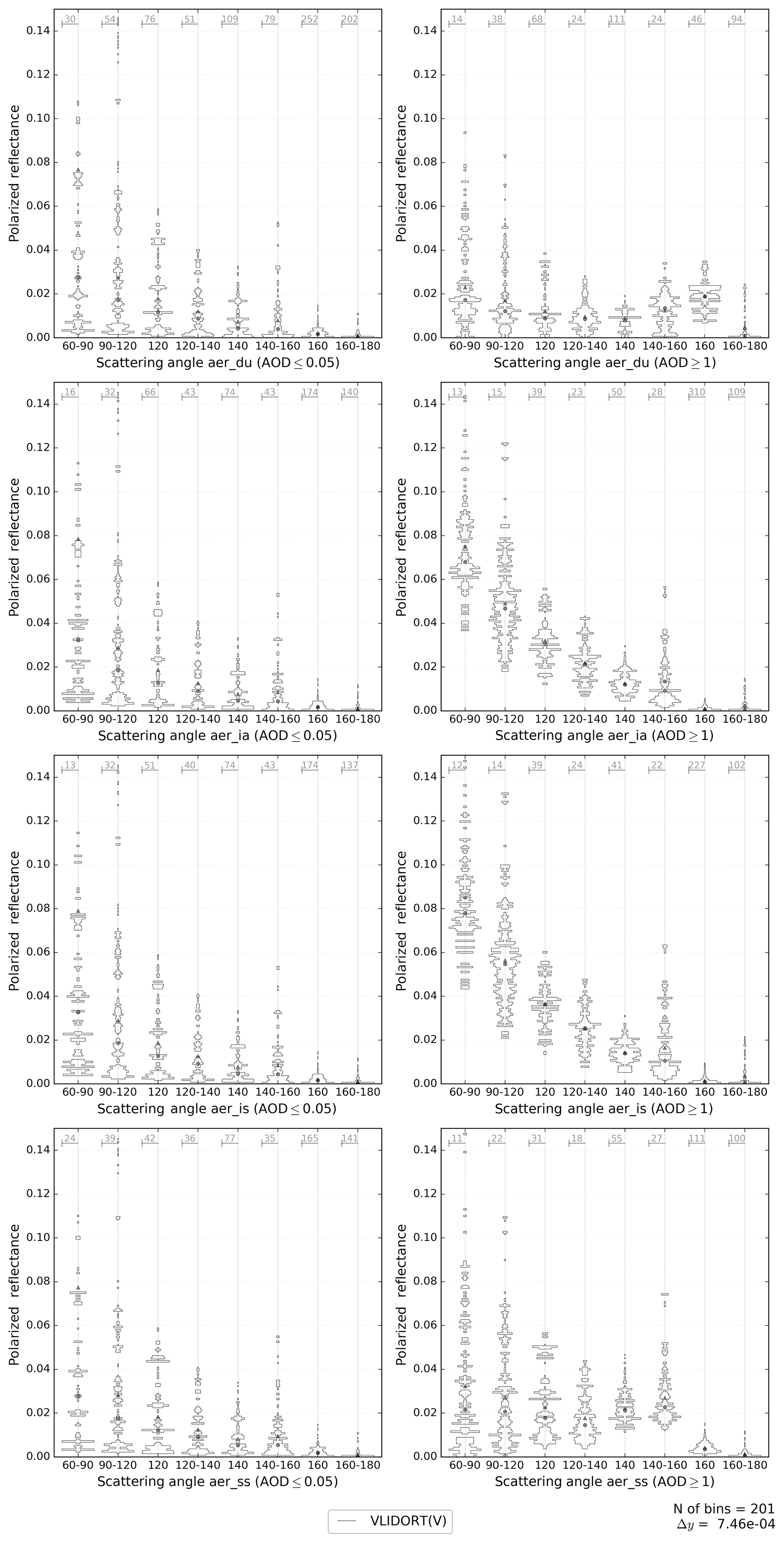
Figure A4Histograms for the polarized reflectance of the VLIDORT (vector) computed reflectances. Only for AOD ≤0.05 in the left column and AOD ≥1 in the right column (AOD at 550 nm). The scattering angle has been binned at intervals with similar quantities of data points. The four aerosol types considered in this work are shown in different panels.
The supplement related to this article is available online at: https://doi.org/10.5194/gmd-12-805-2019-supplement.
JE designed the benchmarking exercise, selected the aerosol models, performed the 6SV2 and DISORT simulations, processed the results, and drafted the manuscript. PD prepared the vertical molecular profiles. OB, JE, LL, and AB performed the Mie calculations. LL performed the VLIDORT simulations. RH designed the FLOTSAM model and performed the corresponding simulations, while AB added FLOTSAM's BRDF capability. All authors contributed to the analysis and the manuscript.
The authors do not declare any competing interest.
The authors acknowledge support from the Copernicus Atmosphere Monitoring
Service implemented by ECMWF on behalf of the European Commission. The
authors thank Didier Tanré for his interesting comments on the draft of the
manuscript. The authors would also like to thank the 6SV2 development team
for their help in resolving small issues with the model and Vijay Natraj and
Robert
Spurr and the two anonymous reviewers for their comments in the
discussion phase. Computing was partly performed on the ESPRI data and
computing centre of the Institut Pierre-Simon
Laplace.
Edited by: Andrea Stenke
Reviewed by: two anonymous referees
Barlakas, V.: A New Three–Dimensional Vector Radiative Transfer Model and Applications to Saharan Dust Fields, PhD thesis, University of Leipzig, 108 pp., 2016. a
Barlakas, V., Macke, A., and Wendisch, M.: SPARTA – Solver for Polarized Atmospheric Radiative Transfer Applications: Introduction and application to Saharan dust fields, J. Quant. Spectrosc. Ra., 178, 77–92, https://doi.org/10.1016/j.jqsrt.2016.02.019, 2016. a
Benedetti, A., Reid, J. S., Knippertz, P., Marsham, J. H., Di Giuseppe, F., Rémy, S., Basart, S., Boucher, O., Brooks, I. M., Menut, L., Mona, L., Laj, P., Pappalardo, G., Wiedensohler, A., Baklanov, A., Brooks, M., Colarco, P. R., Cuevas, E., da Silva, A., Escribano, J., Flemming, J., Huneeus, N., Jorba, O., Kazadzis, S., Kinne, S., Popp, T., Quinn, P. K., Sekiyama, T. T., Tanaka, T., and Terradellas, E.: Status and future of numerical atmospheric aerosol prediction with a focus on data requirements, Atmos. Chem. Phys., 18, 10615–10643, https://doi.org/10.5194/acp-18-10615-2018, 2018. a, b
Bocquet, M., Elbern, H., Eskes, H., Hirtl, M., Žabkar, R., Carmichael, G. R., Flemming, J., Inness, A., Pagowski, M., Pérez Camaño, J. L., Saide, P. E., San Jose, R., Sofiev, M., Vira, J., Baklanov, A., Carnevale, C., Grell, G., and Seigneur, C.: Data assimilation in atmospheric chemistry models: current status and future prospects for coupled chemistry meteorology models, Atmos. Chem. Phys., 15, 5325–5358, https://doi.org/10.5194/acp-15-5325-2015, 2015. a
Bodhaine, B. A., Wood, N. B., Dutton, E. G., and Slusser, J. R.: On Rayleigh optical depth calculations, J. Atmos. Ocean. Tech., 16, 1854–1861, https://doi.org/10.1175/1520-0426(1999)016<1854:ORODC>2.0.CO;2, 1999. a
Chevallier, F., Chéruy, F., Scott, N. A., and Chédin, A.: A neural network approach for a fast and accurate computation of a longwave radiative budget, J. Appl. Meteorol., 37, 1385–1397, https://doi.org/10.1175/1520-0450(1998)037<1385:ANNAFA>2.0.CO;2, 1998. a
Collins, W. D., Rasch, P. J., Eaton, B. E., Khattatov, B. V., Lamarque, J., and Zender, C. S.: Simulating aerosols using a chemical transport model with assimilation of satellite aerosol retrievals: Methodology for INDOEX, J. Geophys. Res.-Atmos., 106, 7313–7336, https://doi.org/10.1029/2000JD900507, 2001. a
Coulson, K., Dave, J. V., and Sekera, Z.: Tables related to radiation emerging from a planetary atmosphere with Rayleigh scattering, Berkeley, U.S., University of California Press, 1960. a
de Haan, J. F., Bosma, P. B., and Hovenier, J. W.: The adding method for multiple scattering calculations of polarized light, Astron. Astrophys., 183, 371–391, 1987. a, b, c
de Rooij, W. A. and van der Stap, C. C. A. H.: Expansion of Mie scattering matrices in generalized spherical functions, Astron. Astrophys., 131, 237–248, 1984. a
Ding, S., Xie, Y., Yang, P., Weng, F., Liu, Q., Baum, B., and Hu, Y.: Estimates of radiation over clouds and dust aerosols: Optimized number of terms in phase function expansion, J. Quant. Spectrosc. Ra., 110, 1190–1198, https://doi.org/10.1016/j.jqsrt.2009.03.032, 2009. a
Drury, E., Jacob, D. J., Wang, J., Spurr, R. J. D., and Chance, K.: Improved algorithm for MODIS satellite retrievals of aerosol optical depths over western North America, J. Geophys. Res.-Atmos., 113, D16204, https://doi.org/10.1029/2007JD009573, d16204, 2008. a
Dubovik, O., Herman, M., Holdak, A., Lapyonok, T., Tanré, D., Deuzé, J. L., Ducos, F., Sinyuk, A., and Lopatin, A.: Statistically optimized inversion algorithm for enhanced retrieval of aerosol properties from spectral multi-angle polarimetric satellite observations, Atmos. Meas. Tech., 4, 975–1018, https://doi.org/10.5194/amt-4-975-2011, 2011. a
Dubuisson, P., Dessailly, D., Vesperini, M., and Frouin, R.: Water vapor retrieval over ocean using near infrared radiometry, J. Geophys. Res.-Atmos., 109, D19106, https://doi.org/10.1029/2004JD004516, 2004. a
Dubuisson, P., Roger, J. C., Mallet, M., and Dubovik, O.: A Code to Compute the Direct Solar Radiative Forcing: Application to Anthropogenic Aerosols during the ESCOMPTE Experiment, A. Deepak Publishing, Hampton, Va, 127–130, 2006. a
Emde, C., Barlakas, V., Cornet, C., Evans, F., Korkin, S., Ota, Y., Labonnote, L. C., Lyapustin, A., Macke, A., Mayer, B., and Wendisch, M.: IPRT polarized radiative transfer model intercomparison project – Phase A, J. Quant. Spectrosc. Ra., 164, 8–36, https://doi.org/10.1016/j.jqsrt.2015.05.007, 2015. a, b, c
Emde, C., Barlakas, V., Cornet, C., Evans, F., Wang, Z., Labonotte, L. C., Macke, A., Mayer, B., and Wendisch, M.: IPRT polarized radiative transfer model intercomparison project – Three-dimensional test cases (phase B), J. Quant. Spectrosc. Ra., 209, 19–44, https://doi.org/10.1016/j.jqsrt.2018.01.024, 2018. a, b, c
Ganapol, B.: A 1D radiative transfer benchmark with polarization via doubling and adding, J. Quant. Spectrosc. Ra., 201, 236–250, https://doi.org/10.1016/j.jqsrt.2017.06.028, 2017. a
Hale, G. M. and Querry, M. R.: Optical Constants of Water in the 200-nm to 200-µm Wavelength Region, Appl. Optics, 12, 555–563, https://doi.org/10.1364/AO.12.000555, 1973. a
Hess, M., Koepke, P., and Schult, I.: Optical Properties of Aerosols and Clouds: The Software Package OPAC, B. Am. Meteorol. Soc., 79, 831–844, https://doi.org/10.1175/1520-0477(1998)079<0831:OPOAAC>2.0.CO;2, 1998. a, b
Hogan, R. J.: Fast reverse-mode automatic differentiation using expression templates in C++, ACM T. Math. Software, 40, 26:1–26:16, 2014. a
Hogan, R. J.: Adept 2.0: a combined automatic differentiation and array library for C++, https://doi.org/10.5281/zenodo.1004730, 2017. a
Hollingsworth, A., Engelen, R. J., Textor, C., Benedetti, A., Boucher, O., Chevallier, F., Dethof, A., Elbern, H., Eskes, H., Flemming, J., Granier, C., Kaiser, J. W., Morcrette, J.-J., Rayner, P., Peuch, V.-H., Rouil, L., Schultz, M. G., Simmons, A. J., and The Gems Consortium: Toward a monitoring and forecasting system for atmospheric composition, B. Am. Meteorol. Soc., 89, 1147–1164, https://doi.org/10.1175/2008BAMS2355.1, 2008. a
Illingworth, A. J., Barker, H. W., Beljaars, A., Chepfer, H., Delanoë, J., Domenech, C., Donovan, D. P., Fukuda, S., Hirakata, M., Hogan, R. J., Huenerbein, A., Kollias, P., Kubota, T., Nakajima, T., Nakajima, T. Y., Nishizawa, T., Ohno, Y., Okamoto, H., Oki, R., Sato, K., Satoh, M., Wandinger, U., and Wehr, T.: The EarthCARE Satellite: the next step forward in global measurements of clouds, aerosols, precipitation and radiation, B. Am. Meteorol. Soc., 96, 1311–1332, 2015. a
Kokhanovsky, A. A., Budak, V. P., Cornet, C., Duan, M., Emde, C., Katsev, I. L., Klyukov, D. A., Korkin, S. V., C-Labonnote, L., Mayer, B., Min, Q., Nakajima, T., Ota, Y., Prikhach, A. S., Rozanov, V. V., Yokota, T., and Zege, E. P.: Benchmark results in vector atmospheric radiative transfer, J. Quant. Spectrosc. Ra., 111, 1931–1946, https://doi.org/10.1016/j.jqsrt.2010.03.005, 2010a. a
Kokhanovsky, A. A., Deuzé, J. L., Diner, D. J., Dubovik, O., Ducos, F., Emde, C., Garay, M. J., Grainger, R. G., Heckel, A., Herman, M., Katsev, I. L., Keller, J., Levy, R., North, P. R. J., Prikhach, A. S., Rozanov, V. V., Sayer, A. M., Ota, Y., Tanré, D., Thomas, G. E., and Zege, E. P.: The inter-comparison of major satellite aerosol retrieval algorithms using simulated intensity and polarization characteristics of reflected light, Atmos. Meas. Tech., 3, 909–932, https://doi.org/10.5194/amt-3-909-2010, 2010b. a
Kopparla, P., Natraj, V., Limpasuvan, D., Spurr, R., Crisp, D., Shia, R.-L., Somkuti, P., and Yung, Y. L.: PCA-based radiative transfer: Improvements to aerosol scheme, vertical layering and spectral binning, J. Quant. Spectrosc. Ra., 198, 104–111, https://doi.org/10.1016/j.jqsrt.2017.05.005, 2017. a
Korkin, S., Lyapustin, A., Sinyuk, A., Holben, B., and Kokhanovsky, A.: Vector radiative transfer code SORD: Performance analysis and quick start guide, J. Quant. Spectrosc. Ra., 200, 295–310, https://doi.org/10.1016/j.jqsrt.2017.04.035, 2017. a, b
Kotchenova, S. Y. and Vermote, E. F.: Validation of a vector version of the 6S radiative transfer code for atmospheric correction of satellite data. Part II. Homogeneous Lambertian and anisotropic surfaces, Appl. Optics, 46, 4455–4464, https://doi.org/10.1364/AO.46.004455, 2007. a, b
Kotchenova, S. Y., Vermote, E. F., Matarrese, R., and Frank J. Klemm, J.: Validation of a vector version of the 6S radiative transfer code for atmospheric correction of satellite data. Part I: Path radiance, Appl. Optics, 45, 6762–6774, https://doi.org/10.1364/AO.45.006762, 2006. a, b, c, d
Krasnopolsky, V. M. and Chevallier, F.: Some neural network applications in environmental sciences. Part II: Advancing computational efficiency of environmental numerical models, Neural Networks, 16, 335–348, https://doi.org/10.1016/S0893-6080(03)00026-1, 2003. a
Lenoble, J., Herman, M., Deuzé, J., Lafrance, B., Santer, R., and Tanré, D.: A successive order of scattering code for solving the vector equation of transfer in the earth's atmosphere with aerosols, J. Quant. Spectrosc. Ra., 107, 479–507, https://doi.org/10.1016/j.jqsrt.2007.03.010, 2007. a
Martin, W., Cairns, B., and Bal, G.: Adjoint methods for adjusting three-dimensional atmosphere and surface properties to fit multi-angle/multi-pixel polarimetric measurements, J. Quant. Spectrosc. Ra., 144, 68–85, https://doi.org/10.1016/j.jqsrt.2014.03.030, 2014. a
Martin, W. G. and Hasekamp, O. P.: A demonstration of adjoint methods for multi-dimensional remote sensing of the atmosphere and surface, J. Quant. Spectrosc. Ra., 204, 215–231, https://doi.org/10.1016/j.jqsrt.2017.09.031, 2018. a, b
McClatchey, R., Fenn, R., Volz, F., and Garing, J.: Optical Properties of the Atmosphere (Revised), Tech. rep., Air Force Cambridge Research Laboratories Hascom AFB, MA, 1971. a
Migliorini, S.: On the equivalence between radiance and retrieval assimilation, Mon. Weather Rev., 140, 258–265, https://doi.org/10.1175/MWR-D-10-05047.1, 2012. a
Mishchenko, M. I. and Travis, L. D.: Satellite retrieval of aerosol properties over the ocean using polarization as well as intensity of reflected sunlight, J. Geophys. Res.-Atmos., 102, 16989–17013, https://doi.org/10.1029/96JD02425, 1997. a, b, c, d
Mishchenko, M. I. and Zakharova, N. T.: Fortran Codes for the Computation of (Polarized) Bidirectional Reflectance of Flat Particulate Layers and Rough Surfaces, available at: https://www.giss.nasa.gov/staff/mmishchenko/brf/, last access: 19 February 2019.
Nakajima, T. and Tanaka, M.: Algorithms for radiative intensity calculations in moderately thick atmospheres using a truncation approximation, J. Quant. Spectrosc. Ra., 40, 51–69, https://doi.org/10.1016/0022-4073(88)90031-3, 1988. a, b
Natraj, V. and Spurr, R. J.: A fast linearized pseudo-spherical two orders of scattering model to account for polarization in vertically inhomogeneous scattering–absorbing media, J. Quant. Spectrosc. Ra., 107, 263- 293, https://doi.org/10.1016/j.jqsrt.2007.02.011, 2007. a
Natraj, V., Li, K.-F., and Yung, Y. L.: Rayleigh scattering in planetary atmospheres: Corrected tables through accurate computation of X and Y functions, Astrophys. J., 691, 1909–1920, 2009. a
Pfreundschuh, S., Eriksson, P., Duncan, D., Rydberg, B., Håkansson, N., and Thoss, A.: A neural network approach to estimating a posteriori distributions of Bayesian retrieval problems, Atmos. Meas. Tech., 11, 4627–4643, https://doi.org/10.5194/amt-11-4627-2018, 2018. a
Pincus, R. and Evans, K. F.: Computational cost and accuracy in calculating three-dimensional radiative transfer: Results for new implementations of Monte Carlo and SHDOM, J. Atmos. Sci., 66, 3131–3146, https://doi.org/10.1175/2009JAS3137.1, 2009. a
Remer, L. A., Kaufman, Y. J., Tanré, D., Mattoo, S., Chu, D. A., Martins, J. V., Li, R.-R., Ichoku, C., Levy, R. C., Kleidman, R. G., Eck, T. F., Vermote, E., and Holben, B. N.: The MODIS aerosol algorithm, products, and validation, J. Atmos. Sci., 62, 947–973, https://doi.org/10.1175/JAS3385.1, 2005. a
Scheck, L., Frèrebeau, P., Buras-Schnell, R., and Mayer, B.: A fast radiative transfer method for the simulation of visible satellite imagery, J. Quant. Spectrosc. Ra., 175, 54–67, https://doi.org/10.1016/j.jqsrt.2016.02.008, 2016. a, b
Siewert, C.: A concise and accurate solution to Chandrasekhar's basic problem in radiative transfer, J. Quant. Spectrosc. Ra., 64, 109–130, https://doi.org/10.1016/S0022-4073(98)00144-7, 2000a. a
Siewert, C.: A discrete-ordinates solution for radiative-transfer models that include polarization effects, J. Quant. Spectrosc. Ra., 64, 227–254, https://doi.org/10.1016/S0022-4073(99)00006-0, 2000b. a
Somkuti, P., Boesch, H., Natraj, V., and Kopparla, P.: Application of a PCA-Based Fast Radiative Transfer Model to XCO2 Retrievals in the Shortwave Infrared, J. Geophys. Res.-Atmos., 122, 10477–10496, https://doi.org/10.1002/2017JD027013, 2017. a
Spurr, R.: LIDORT and VLIDORT: Linearized pseudo-spherical scalar and vector discrete ordinate radiative transfer models for use in remote sensing retrieval problems, Springer Berlin Heidelberg, Berlin, Heidelberg, https://doi.org/10.1007/978-3-540-48546-9_7, 229–275, 2008. a, b
Spurr, R.: VLIDORT User's Guide, version 2.7, Tech. rep., RT Solutions, Inc., 2014. a
Stamnes, K. and Swanson, R. A.: A new look at the Discrete Ordinate Method for radiative transfer calculations in anisotropically scattering atmospheres, J. Atmos. Sci., 38, 387–399, https://doi.org/10.1175/1520-0469(1981)038<0387:ANLATD>2.0.CO;2, 1981. a
Stamnes, K., Tsay, S.-C., Wiscombe, W., and Jayaweera, K.: Numerically stable algorithm for discrete-ordinate-method radiative transfer in multiple scattering and emitting layered media, Appl. Optics, 27, 2502–2509, https://doi.org/10.1364/AO.27.002502, 1988. a, b
Tanré, D., Bréon, F. M., Deuzé, J. L., Dubovik, O., Ducos, F., François, P., Goloub, P., Herman, M., Lifermann, A., and Waquet, F.: Remote sensing of aerosols by using polarized, directional and spectral measurements within the A-Train: the PARASOL mission, Atmos. Meas. Tech., 4, 1383–1395, https://doi.org/10.5194/amt-4-1383-2011, 2011. a
Toon, O. B. and Ackerman, T. P.: Algorithms for the calculation of scattering by stratified spheres, Appl. Optics, 20, 3657–3660, https://doi.org/10.1364/AO.20.003657, 1981. a
Toon, O. B., McKay, C. P., Ackerman, T. P., and Santhanam, K.: Rapid calculation of radiative heating rates and photodissociation rates in inhomogeneous multiple scattering atmospheres, J. Geophys. Res., 94, 16287–16301, 1989. a
Vermote, E., Tanré, D., Deuzé, J.-L., Herman, M., and Morcrette, J.-J.: Second Simulation of the Satellite Signal in the Solar Spectrum, 6S: An overview, IEEE T. Geosci. Remote, 35, 675–686, 1997. a
Wang, C., Yang, P., Nasiri, S. L., Platnick, S., Baum, B. A., Heidinger, A. K., and Liu, X.: A fast radiative transfer model for visible through shortwave infrared spectral reflectances in clear and cloudy atmospheres, J. Quant. Spectrosc. Ra., 116, 122–131, https://doi.org/10.1016/j.jqsrt.2012.10.012, 2013a. a
Wang, C., Yang, P., Platnick, S., Heidinger, A. K., Baum, B. A., Greenwald, T., Zhang, Z., and Holz, R. E.: Retrieval of Ice Cloud Properties from AIRS and MODIS Observations Based on a Fast High-Spectral-Resolution Radiative Transfer Model, J. Appl. Meteorol. Clim., 52, 710–726, https://doi.org/10.1175/JAMC-D-12-020.1, 2013b. a
Wang, J., Xu, X., Spurr, R., Wang, Y., and Drury, E.: Improved algorithm for MODIS satellite retrievals of aerosol optical thickness over land in dusty atmosphere: Implications for air quality monitoring in China, Remote Sens. Environ., 114, 2575–2583, https://doi.org/10.1016/j.rse.2010.05.034, 2010. a
Wang, J., Xu, X., Henze, D. K., Zeng, J., Ji, Q., Tsay, S.-C., and Huang, J.: Top-down estimate of dust emissions through integration of MODIS and MISR aerosol retrievals with the GEOS-Chem adjoint model, Geophys. Res. Lett., 39, L08802, https://doi.org/10.1029/2012GL051136, 2012. a
Weaver, C., da Silva, A., Chin, M., Ginoux, P., Dubovik, O., Flittner, D., Zia, A., Remer, L., Holben, B., and Gregg, W.: Direct insertion of MODIS radiances in a global aerosol transport model, J. Atmos. Sci., 64, 808–827, https://doi.org/10.1175/JAS3838.1, 2007. a
Weng, F.: Advances in Radiative Transfer Modeling in Support of Satellite Data Assimilation, J. Atmos. Sci., 64, 3799–3807, https://doi.org/10.1175/2007JAS2112.1, 2007. a
Wiscombe, W. J.: Improved Mie scattering algorithms, Appl. Optics, 19, 1505–1509, https://doi.org/10.1364/AO.19.001505, 1980. a
Woodward, S.: Modeling the atmospheric life cycle and radiative impact of mineral dust in the Hadley Centre climate model, J. Geophys. Res.-Atmos., 106, 18155–18166, https://doi.org/10.1029/2000JD900795, 2001. a
Xu, X., Wang, J., Henze, D. K., Qu, W., and Kopacz, M.: Constraints on aerosol sources using GEOS–Chem adjoint and MODIS radiances, and evaluation with multisensor (OMI, MISR) data, J. Geophys. Res.-Atmos., 118, 6396–6413, https://doi.org/10.1002/jgrd.50515, 2013. a