the Creative Commons Attribution 4.0 License.
the Creative Commons Attribution 4.0 License.
 | 08 Mar 2019
LPJ-GM 1.0: simulating migration efficiently in a dynamic vegetation model
Michael Mischurow
Erik Lindström
Dörte Lehsten
Heike Lischke
Dynamic global vegetation models are a common tool to assess the effect of climate and land use change on vegetation. Though most applications of dynamic global vegetation models use plant functional types, some also simulate species occurrences. While the current development aims to include more processes, e.g. the nitrogen cycle, the models still typically assume an ample seed supply allowing all species to establish once the climate conditions are suitable. Pollen studies have shown that a number of plant species lag behind in occupying climatological suitable areas (e.g. after a change in the climate) as they need to arrive at and establish in the newly suitable areas. Previous attempts to implement migration in dynamic vegetation models have allowed for the simulation of either only small areas or have been implemented as a post-process, not allowing for feedbacks within the vegetation. Here we present two novel methods simulating migrating and interacting tree species which have the potential to be used for simulations of large areas. Both distribute seeds between grid cells, leading to individual establishment. The first method uses an approach based on fast Fourier transforms, while in the second approach we iteratively shift the seed production matrix and disperse seeds with a given probability. While the former method is computationally faster, it does not allow for modification of the seed dispersal kernel parameters with respect to terrain features, which the latter method allows.
We evaluate the increase in computational demand of both methods. Since dispersal acts at a scale no larger than 1 km, all dispersal simulations need to be performed at maximum at that scale. However, with the currently available computational power it is not feasible to simulate the local vegetation dynamics of a large area at that scale. We present an option to decrease the required computational costs through a reduction in the number of grid cells for which the local dynamics are simulated only along migration transects. Evaluation of species patterns and migration speeds shows that simulating along transects reduces migration speed, and both methods applied on the transects produce reasonable results. Furthermore, using the migration transects, both methods are sufficiently computationally efficient to allow for large-scale DGVM simulations with migration.
- Article
(3561 KB) -
Supplement
(694 KB) - BibTeX
- EndNote


A large suite of dynamic global vegetation models (DGVMs) is currently used to simulate the effects of climate and/or land use change on vegetation and ecosystem properties. These simulations result in projections (or hindcasts) of species ranges as well as changes in ecosystem properties such as carbon stocks and fluxes. Examples of these DGVMs include ORCHIDEE (Yue et al., 2018), LPJ-GUESS (Sitch et al., 2003), and IBIS (Foley et al., 1998; Sato et al., 2007); for a review of DGVM features, see Quillet et al. (2010).
While most DGVM applications use plant functional types (groups of plant species with similar traits and responses to environmental conditions), here we only consider applications which explicitly simulate tree species (e.g. Hickler et al., 2012). These models typically assume that species can establish at any site once the environmental conditions become suitable. However, in real ecosystems species not only need to establish and replace existing vegetation, which the processes in gap models describe successfully, but they also need to have a sufficient amount of seeds present at a given location to successfully establish. Implicitly, current DGVMs assume that ample amounts of seeds of all species are present in every location.
While this approach might seem reasonable in cases in which the vegetation can keep up with climate change (i.e. moving sufficiently fast to occupy areas which become suitable), there have been a number of instances reported in which a considerable migration lag occurred. For instance, Fagus sylvatica has been shown to have a considerable migration lag and is currently still in the process of occupying its climatological optimum (Bradshaw and Lindbladh, 2005).
The implementation of migration into dynamic vegetation models is not only of interest for the simulation of historical species ranges, but it is also of interest for the projection of ecosystem properties in the future since migration lags might lead to uncertainties in projected ecosystem properties if the wrong species community is predicted to occur at a certain site (Neilson et al., 2005). Especially, given that the speed at which environmental conditions change is currently unprecedented, at least over the last centuries, effects of the migration lag of key species should be evaluated when projecting ecosystem properties. This holds in particular for projections over several centuries. For periods of less than 50–100 years ahead, which corresponds to at most a few generations of most tree species, the explicit modelling of seed dispersal might be less important for simulating tree distributions, in particular when taking into account the overwhelming influence of human activities.
Migration lags can be caused by different factors. Seed transport might only occur over limited distances. But low seed amounts and, in particular, long generation times can also slow down migration. Seed amount and generation time depend on the competition with other trees: a free-standing tree starts to produce seeds earlier and produces more than a tree of the same age in a closed forest. The competitors, however, are also migrating, which leads to feedbacks between the species (Snell et al., 2014).
Thus, for simulations over large areas covering long time spans, species migration – consisting of (a) local dynamics influenced by the environment, (b) competition between species, and (c) seed dispersal – has to be taken into account simultaneously for several species.
Species migration has been implemented successfully in dynamic vegetation models working on smaller extents and finer scales than DGVMs typically use, e.g. forest landscape models (FLMs; review in Shifley et al., 2017) such as TreeMig, (Lischke et al., 2006), LandClim (Schumacher et al., 2004), Landis (Mladenoff, 2004), and Iland (Seidl et al., 2012) or spatially explicit individual-based models such as LAVESI (Kruse et al., 2018).
In these models, seed dispersal is modelled in a straightforward way: seeds are distributed from each producing to each receiving cell with a distance-dependent probability. However, transferring these approaches to DGVMs is problematic due to a number of conceptual and technical difficulties. DGVMs usually operate on a coarse spatial resolution to reduce computational load and input data requirements. This neglects the spatial heterogeneity within the grid cells. Additionally, and even more critical for implementing migration, it leads to discretization errors: if it is assumed that the forest representing the grid cell is located in the centre of the cell, the seeds cannot move far enough to leave the cell (given a typical cell size of 50 km×50 km or 10 km×10 km). If, on the other hand, a uniformly distributed forest in the cell is assumed in the simulation some seeds reach the neighbour cell with each time step, leading to a resolution-dependent speed-up of migration.
Also, some specifics of model implementations might complicate the inclusion of migration in some DGVMs. Many DGVM implementations are done in a way that for each grid cell all years are simulated before the simulation of the next cell is started. This is done to minimize input–output effort since all climate data for each cell are read in at once and it also eases parallelization for multicore computers, since in this case each node is assigned a number of grid cells which the node calculates independently of the other nodes without communication. However, for simulating seed dispersal, all cells need to be annually evaluated. In addition to the reasons mentioned before, most DGVM applications use plant functional types, which typically comprise species with very different traits with respect to migration (e.g. dispersal vectors or seed properties). Hence, introducing migration would require splitting up PFTs into smaller groups and parameterizing the additional properties.
There have been a number of attempts to integrate species migration in DGVMs (see Snell et al., 2014, and the Discussion section). For example, Sato and Ise (2012) developed a DGVM in which species could potentially migrate between neighbouring cells with a fixed rate of about 1 km yr−1, while Snell (2014) simulated migration as an infection process between patches and within each grid cell.
However, to the knowledge of the authors, there is no implementation of a migration scheme into a DGVM which allows for simulations with a large extent, takes migration within the grid cell into account, and includes feedbacks between all simulated species.
Here we present two methods to fill this gap, i.e. allow for the simultaneous simulation of the migration of several species. The methods are implemented into the LPJ-GUESS DGVM but can potentially also be implemented into other DGVMs. Though they are tested here using a virtual landscape, they can be applied for simulations of large areas given current computing resources.
2.1 The dynamic vegetation model LPJ-GUESS
LPJ-GUESS is a flexible framework for modelling the dynamics of terrestrial ecosystems from landscape to global scales (Sitch et al., 2003; Smith et al., 2001). Similar to most other DGVMs, it requires time series of climate data (precipitation, air temperature, and shortwave radiation), soil conditions, and carbon dioxide concentrations as input and explicitly simulates vegetation cover. While it uses plant functional types in most applications, some applications simulate tree species (e.g. Hickler et al., 2012; Lehsten et al., 2015). LPJ-GUESS explicitly simulates canopy conductance, photosynthesis, phenology, and carbon allocation. It uses a detailed individual-based representation of forest stand structure and dynamics. Each species (or PFT) has a specific growth form, leaf phenology, life history, and bioclimatic limits determining its performance and competitive interactions under the forcing conditions and realized ecosystem state of a particular grid cell (Sitch et al., 2003). A large body of publications describes the features of LPJ-GUESS in detail; here we concentrate on the changes that were applied to LPJ-GUESS version 4.0 (Lindeskog et al., 2013; Smith et al., 2014). To differentiate between the original version of LPJ-GUESS and our extended version (in which we implemented the migration module) we refer to the extended version as LPJ-GM (short for LPJ-GUESS-MIGRATION).
2.2 Technical implementation
Standard LPJ-GUESS simulations are typically performed at a computing cluster with cells running on different nodes of the cluster without any interaction of the nodes. We implemented a distributed simulation using a message-passing interface (MPI) (Clarke et al., 1994) with the grid cells communicating with a master process.
Seeds are potentially produced in each grid cell at the end of each year after the first 100 years (see below). The number of seeds produced is sent to the node computing the dispersal, while all nodes wait for this master node to finish the calculation. This node sends the number of seeds that arrive at each grid cell back to all nodes to continue the calculation.
Similar to the standard version of LPJ-GUESS (Sitch et al., 2003; Smith et al., 2001), in the first 100 years no seed dispersal is performed and all species are allowed to establish and grow without seed limitation and without N limitation to equilibrate the soil pools with carbon and nitrogen. This time period is used to sample NPP given a certain N deposition and climate to subsequently equilibrate the N pools of the soil and a fast spin-up of 40 000 years approximated using the sampled rates of C assimilation (Smith et al., 2014). After this initialization period all vegetation is killed and succession starts from a bare soil with seed limitation active. In LPJ-GM seed dispersal is done on an annual basis. The amount of seeds produced is communicated to the master node at the end of each year. The master node redistributes seeds over the whole spatial domain according to the dispersal algorithm and communicates the amounts of arriving seeds back to each grid cell. Seeds transferred to the grid cells are added to the seed bank, which determines establishment probability in environmentally suitable cells (environmental suitability is determined by means of environmental envelopes containing, amongst others, minimum survival and establishment temperatures; see Smith et al., 2001). All communications between the processes are done via MPI protocol (Clarke et al., 1994).
LPJ-GUESS is a gap model with the typical successional vegetation changes. To even out successional-based fluctuations in ecosystem properties and to simulate disturbances, most previous applications simulate a certain number of replicate patches per grid cell. All patches share the same climate but potentially differ in their successional stage due to different timing of disturbances and stochastic mortality. Conceptually, each patch has a size of 1000 m2 but represents an area depending on the resolution of the grid cell. Patches have no spatial position with respect to each other and do not interact (Smith et al., 2001). In LPJ-GM we reduced the number of patches to one but achieved the representative averaging by using explicitly placed small grid cells instead of statistical units (replicate patches). For each large grid cell in the climate grid we simulate a large number of cells of 1 km2 area, resulting in a more than sufficient averaging of successional stages. LPJ-GUESS simulations are typically performed with patch numbers around 10 (e.g. Smith et al., 2001), but depending on the aim of the simulation patch numbers have even been increased to 500 (e.g. Lehsten et al., 2016). In our set-up even with 50 km corridors LPJ-GM represents a 0.5×0.5∘ cell with 200 simulation cells ranging at the higher end of the patch number per area compared to previous simulations. We demonstrate this in Fig. 3 in which a single large grid cell is separated into 11×11 small grid cells with the same climate, each of which is 1 km×1 km. The local dynamics and seed production are only simulated along the transects (grey or green cells in left panel of Fig. 3). As a next step the seed production is interpolated onto all cells for which no local dynamics were calculated, and the seed dispersal is simulated. Finally, seedling establishment is simulated, but only in the grid cells on the corridors (more details for the different steps are given below).
2.3 Migration processes
2.3.1 Seed production
The seed production starts once the tree reaches maturity height and is scaled linearly with leaf area up to maximum (LAI). The seed number produced per tree is calculated as the product of the maximum fecundity multiplied by the proportion of the current LAI to the maximum LAI and multiplied by the area per grid cell. For example, the maximum fecundity of beech is 29 000, the maximum LAI is 5 m2 m−2, and the maturity height is 14.4 m. Hence, a tree of 15 m height is above the maturity height, and with an LAI of 2.5 m2 m−2 it will produce seeds. No specific age of maturity is taken into account.
All seeds of a species produced at a location within a year are available for seed dispersal. Once seeds have entered the seed bank, no further dispersal is possible (they remain in the seed bank). Though LPJ-GUESS keeps track of carbon allocated to the main plant compartments and even allocates a certain amount of carbon to seeds (which is transferred to the litter pool, the soil pool, and finally the atmosphere), for simplicity we decided not to relate the seed production to the carbon accounting at this point. Allocation rules, including seed production and even mast fruiting effects (synchronized strong increases in seed production e.g. similar to Lischke et al., 2006), could be included in the future.
2.3.2 Seed dispersal
The produced seeds are distributed according to
is the seed production, and the seed dispersal kernel in Euclidean coordinates. The seed distribution Sd(x,y), i.e. the input of seeds in location x, y, is then obtained by integrating over all possible locations for arriving at x,y.
Thus, the seed distribution is given by the convolution of the seed production and the seed dispersal kernel:
For this study we used the seed dispersal kernel and parameterization for Fagus sylvatica from TreeMig (Lischke et al., 2006). The seed dispersal kernel defines the probability of seeds arriving at a sink cell (x,y) from the source cell with a certain distance .
The kernel is specified in a polar coordinate system, ks(zθ)=ks(z|θ)ks(θ), with the radial distance z. The seeds follow a mixture of two exponential distributions, the short- and the long-term dispersal, while the angular dispersion, θ, is uniform in all directions (in our case the angular dispersion θ is uniform, but if one is interested e.g. in implementing wind directions this can be changed). Thus, the radial component of the kernel is given by
while the angular term is given by
The dispersal kernel is defined by the species-specific values for the proportion of long-distance dispersal κ and the species expected dispersal distances αs,1 and αs,2 for the two kernels.
The species-specific values for these parameters (0.99 for κs and 25 and 200 m for the two mean dispersal distances ks for Fagus sylvatica) were taken from by Lischke et al. (2006).
2.3.3 Seed bank dynamics
The number of the seeds in the seed bank (i.e. the dormant seeds in the soil that can germinate in subsequent years in each cell) is increased by the influx Sd of seeds according to Eq. (1) and reduced by the yearly loss of germinability (caused by the decay of seeds; see Supplement S4 for parameter values) and the amount of germinated seeds at the end of each simulated year, similar to TreeMig (Lischke et al., 2006).
For each grid cell and each year we prescribe whether the species requires seeds to establish. By not requiring seeds for establishment we define refugia, or we stipulate that the species' seeds are known to be very far dispersed and hence no explicit simulation of establishment by seeds is required for this species. Technically this is implemented by reading in a list for each cell containing a year starting from which species establishment is not limited by the availability of seeds.
2.3.4 Germination
LPJ-GUESS is a gap model and in the original version the number of newly established saplings only depends on the amount of light reaching the forest floor (given that the cell has a suitable climate). In LPG-GM we additionally limit the establishment of seedlings depending stochastically on the number of available seeds. Hence, the seed limitation is applied before the light limitation. The probability that a species establishes is given in Eq. (5).
Pest is the probability of the species establishing, S is the number of seeds, and Pgerm is the seed germination proportion. The extra parameter px takes (implicitly) the area of each grid cell into account. In our case we fixed this parameter to 0.01 after initial testing. Hence, if in a certain year 100 seeds are in the seed bank and the germination rate is 0.71 (value for Fagus sylvatica) the probability of establishment is .
2.4 Enhanced dispersal simulation
One way to simulate seed dispersal is to calculate the convolution of the matrix containing the seed production and the seed dispersal kernel (specified in Eqs. 1 and 3). However, evaluating the convolution explicitly can be computationally expensive for seed dispersal kernels with a long range.
2.4.1 Fast Fourier transform method (FFTM)
An alternative is based on the convolution theorem and the fast Fourier transform (FFT), a technique commonly used in physics, image processing, and engineering (Strang, 1994), but rarely in ecology; see e.g. Powell (2001), Shaw et al. (2006), and Pueyo et al. (2008).
This approach carries out the computations in the frequency domain; see Gonzales and Woods (2002). Here we use the notation to denote the two-dimensional Fourier transform of S and correspondingly F{ks}, the two-dimensional Fourier transform of ks. It then follows that the Fourier transform of the convolution equals the product of the Fourier transforms.
Thus, it is possible to compute the convolution by applying the inverse Fourier transform to the products of the Fourier transforms.
This equation must be discretized before evaluating it on a computer. The discrete Fourier transform is computed using the fast Fourier transform (Cooley and Tukey, 1965), which has a computational cost of O(N2log 2(N)) in two dimensions. The discrete approximation of Sd is then given by
where ⊙ is the element-wise (Hadamard product) multiplication of matrices.
Nowadays, software packages for FFT typically only compute positive frequencies. That means that we have to shift the frequencies prior to the element-wise multiplication of F{S} and F{ks} This is illustrated in Fig. 1; see also Supplement S2.
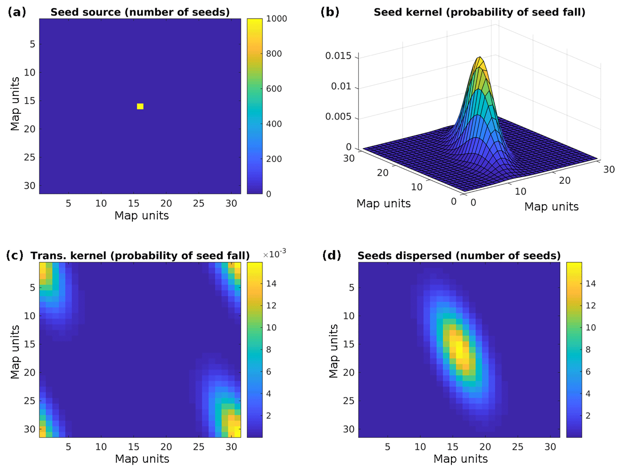
Figure 1(a) Seed source. (b) Example of a seed dispersal kernel (here a non-symmetric kernel is assumed), (c) transformed seed dispersal kernel, and (d) seed distribution after convolution.
While this method allows for the inclusion of different wind distributions by changing the seed dispersal kernel (as long as they are valid for the whole simulated area), it does not allow us to use different seed dispersal kernels at different locations, e.g. due to prevailing wind directions in valleys, due to barriers to animal transport like a motorway, or due to lower transport permeability in already forested areas.
2.4.2 Seed matrix shifting method (SMSM)
Another way to simulate seed dispersal is to simulate the seed movement between the cells explicitly by shifting the matrix containing the produced seeds by one position (repeatedly in all directions of the Moore neighbourhood; i.e. the surrounding eight cells) and simulating the transport of a certain proportion of the seeds into the next cell. Each move can be viewed as an independent random variable. Repeating these moves thus corresponds to a random walk process. The Lindeberg condition for sequences for sums of independent random variables ensures that the kernel will be Gaussian under general conditions (Shiryaev, 2016), with the expected value given by the sum of expected values for each random variable and similarly for the variance (see Supplement S1 for a formal proof and a derivation of the parameters of the resulting normal distribution).
If this is done repeatedly it allows for an easy implementation of spatial explicit differences in seed dispersal kernel distributions by adjusting the proportions of seeds being transported into the next cell according to a similarly sized matrix containing the area roughness or permeability. Through this approach, barriers and even wind speeds in latitudinal and longitudinal directions can be implemented by adjusting the dispersal probabilities accordingly. After the distribution of the dispersed seeds is calculated, the seeds are added to the seed bank. An example calculation of the first three steps of the SMSM (in the final simulation 10 steps are performed) is given in the Supplement S3.
2.5 Corridors
Seed dispersal acts at a rather fine scale compared to the usual scale at which DGVMs are run (LPJ-GUESS is typically run at a 0.5 to 0.1∘ longitude–latitude scale), though some regional applications use finer grids (e.g. Scherstjanoi et al., 2014). Given that the average long-distance seed dispersal, for example for Fagus sylvatica, is 200 m (representing 0.002∘ longitude–latitude at the Equator), simulations at such a coarse scale will not be able to capture this process.
As a compromise between currently available computing resources and required simulation detail we choose a 1 km scale at which we performed our simulations. However, even at this scale, simulating large areas, for example within the European continent, would result in a high computational effort.
Given that in some areas the landscape is rather homogenous while other areas have a variable terrain (or land use conditions), we test whether for homogenous landscapes it is sufficient to simulate the local dynamics only in latitudinal, longitudinal, and diagonal transects (i.e. north–south, east–west, northeast–southwest, and northwest–southeast corridors) and how this will influence the migration speed. The corridors are one grid cell wide and regularly placed in the simulation domain. Their density can be chosen by defining the distance between the latitudinal and longitudinal corridors.
Although LPJ-GM only simulates local dynamics in the cells along the corridors, the seed matrix needed to be filled for the dispersal calculation using the FFTM or the SMSM algorithm. We applied a nearest-neighbour interpolation of the seed production before performing the seed dispersal calculation (theoretical considerations show that a distance-weighted average would strongly speed up the migration).
2.6 Simulation experiments
To test our newly developed migration module we simulated the spread of a single late successional species (Fagus sylvatica) through an area covered by an early successional species (Betula pendula). The species-specific parameters for both species are given in the Supplement S4. All grid cells and all years in the simulated area had a static climate suitable for both species. Though the simulated domain is quadratic in our case, it could have any shape. Each cell in the simulated domain has been simulated independently (except for the influx and outflux of seeds) from the others. For one specific simulation using the SMSM method we assumed differences in the dispersal ability (e.g. more or less permeable areas or physical barriers), while the climate on all grid cells is still static and favourable. The differences in tree dispersal ability from landscape barriers are displayed in Fig. 2. Areas coloured white have zero permeability, and hence no seeds can reach these areas.

Figure 2Seed dispersal permeability for SMSM simulation tests. Each time the seed matrix is shifted, the probability of entering the new cell (which in our test is set to ) is multiplied with the seed dispersal permeability of the new potentially entered cell. A permeability value of 1 indicates that the landscape is not hindering the species-specific seed dispersal, while a value of 0 indicates that the landscape completely blocks any seed movement.
Figure 3 demonstrates the sequence of simulating vegetation dynamics on the corridors, interpolation of seed production, and seed dispersal on the entire grid and back via the seed input on the transects.
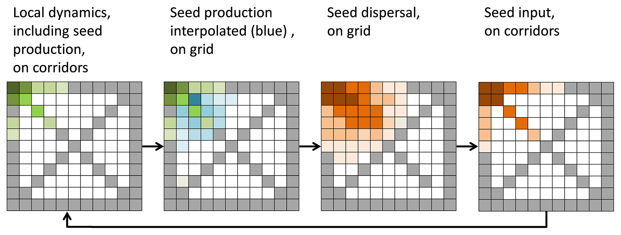
Figure 3Example of a simulated grid with transects (grey). In each time step the local vegetation dynamics, including the seed production (green), is calculated on the transects. Then the seed production of each species is interpolated from the transects to all non-transect grid cells (blue) and then dispersed on the entire grid (brown). The seed input on the transect cell then enters the local dynamics in the next time step.
Given the uniformity of the climate, there should be no variability in the migration speed caused by differences in climatic conditions. We simulated the spread of F. sylvatica from a single grid cell in the corner of the study area, which represents the refugium. We tested several corridor distances (between the parallel and between the diagonal corridors) for their effect on the migration speed. To calculate the migration speed we first determined the migration distance. This was the distance between the start point of the migration and the 95th percentile farthest point in the virtual landscape where the leaf area index (LAI) of F. sylvatica was larger than 0.5. This migration distance was subsequently divided by the simulated time elapsed since the start of the migration. To avoid founder effects we neglected all points within first 5 km from the starting location (the refugium). The simulations were performed over 3000 years and over an area of 100×100 cells of 1 km2. Finally, we ran one simulation in which we did not calculate the seed dispersal (but performed all communication between cells and one run even without the communication), hence allowing us to estimate the computation time demand for the seed dispersal calculation.
2.7 Performance evaluations
To estimate the performance of our methods against an implementation in which all grid cells exchange seeds with each other, we developed a MATLAB® script, since initial testing had shown that such a procedure would be too slow to be implemented in LPJ-GUESS. Hence, when evaluating the performance differences from the script one has to bear in mind that these are calculated in a different environment. However, in a general sense we can see no reason why they should not reflect the performance differences between the algorithms. The whole MATLAB® script testing the performance, including the graphs, is part of the Supplement.
3.1 Explicit seed dispersal
The study comparing the performance of different migration mechanisms without the vegetation dynamics, implemented in MATLAB®, has shown that both the FFTM and the SMSM performed faster than the explicit dispersal from all grid cells to each other within the range of the dispersal (Fig. S2.6 in Supplement S2). This was especially pronounced if the area to be simulated was increased. Though faster than the explicit dispersal method, the SMSM was still up to an order of magnitude slower than the FFTM, in particular for large simulation domains in MATLAB®, while the FFTM and the SMSM required relatively similar amounts of time in the implementation in LPJ-GUESS (Table 1).
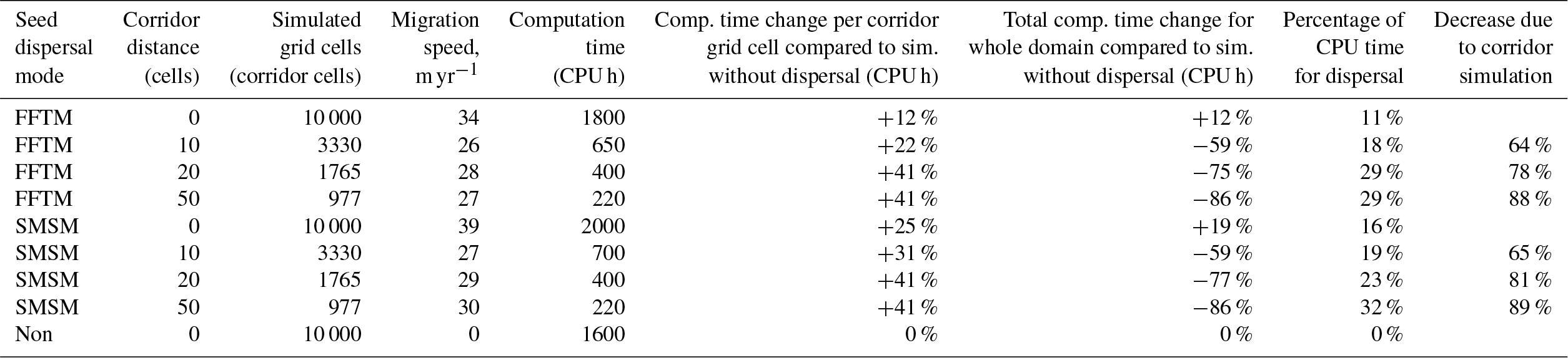
Table 1Summary of migration speeds and calculation time. A corridor distance of 0 indicates no corridors but an area completely filled with grid cells. The simulated grid cell column lists the number of cells for which LPJ-GM calculates the population dynamics; in all simulations the simulation domain (for which the seed dispersal was calculated) had a size of 10 000 grid cells and all simulations were performed over 3000 years. The last line lists a simulation identical to the others except that no seed dispersal was calculated to allow for the estimation of the computation time demand for this operation.
3.2 FFTM simulations
Using the parameterization from TreeMig in a complete (no corridors) simulation area of 100×100 grid cells with a size of 1 km2 each resulted in a migration speed of 34 m per year for Fagus sylvatica (Fig. 4).
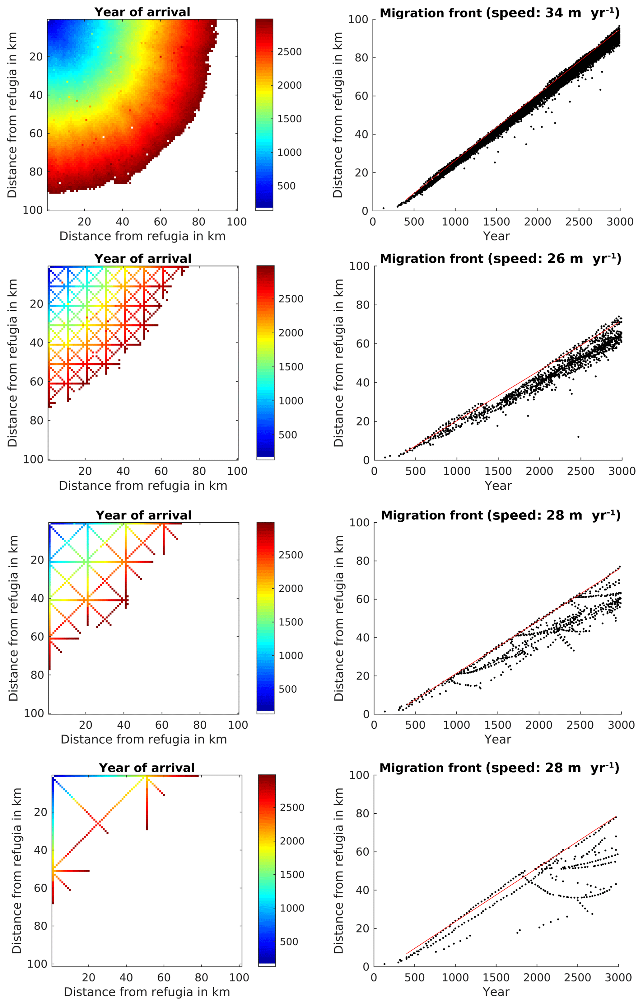
Figure 4Spread of Fagus sylvatica through an area of 100×100 grid cells with static climate using the FFTM algorithm with no corridors or corridors every 10 km, 20 km, or 50 km. The left panels display the time when F. sylvatica first reached an LAI of 0.5. F. sylvatica is allowed to establish freely only in the upper left corner. The right panels show the distance of the grid cells with LAI 0.5 for F. sylvatica from the starting point. The red line indicates the 95th percentile of the grid cells farthest away from the starting point. The migration speed is calculated as slope of this line, taking only grid cells at least 5 km away from the starting point into account to avoid some initial establishing effects.
Though the establishment in the model is stochastic, the simulated spread was relatively smooth. The corridor distances of 10, 20, and 50 km resulted in a reduced migration rate of 26, 28, and 28 m yr−1 (compared to a simulation without corridors), respectively (Fig. 4, lower three rows of panels). While in the simulation without corridors the variability of the migration speed was relatively low (dots under the red line in the upper left panel of Fig. 4), this variability was strongly increased when corridors were simulated. This was caused by F. sylvatica migrating along the diagonal, reaching the endpoint of the diagonal, and then migrating along the longitudinal and latitudinal corridors into cells which actually had a shorter distance to the refugia than the endpoint of the diagonal.
The simulation time per grid cell in the whole area (range for which the seed dispersal was computed) was increased by 12 % by simulating the FFTM, but by using the corridors it was reduced to 36 %, 22 %, and 12 % compared to simulating the full area (Table 1, col. 7). The proportion of computation time used to perform the FFTM increased from 11 % without corridors to 18 %, 29 %, and 29 % for simulations with corridors every 10, 20, and 50 km. This estimate only includes the required time for computing the FFT-based seed dispersal since the control run without seed dispersal still contained all communication between cells. For the control run seeds were produced and sent to the master but the master did not compute the seed dispersal, though it still communicated with all other nodes to allow for a fair assessment of the computation time demand of the two methods (see Table 1). An additional run without any communication resulted in a computation time similar to the run with communication.
3.3 Shifting seed simulations
Initial testing of the probability parameter for the SMSM suggested a value of to generate a migration speed comparable to the migration speed for the FFTM based on the TreeMig parameterization. Using the derivation presented in Supplement S2, it is possible to calculate this parameter for a Gaussian dispersal kernel. One can approximate any dispersal kernel by adding several Gaussian kernel; however, this would increase calculation time since the SMSM would have to be performed several times. Therefore, we decided to choose a parameter for the SMSM approximating the migration speed rather than the seed dispersal kernel used in Lischke et al. (2006). This resulted in a migration speed of 39 m yr−1 for the filled area and 27, 29, and 30 m yr−1 for the 10, 20, and 50 km corridors (Fig. 5).
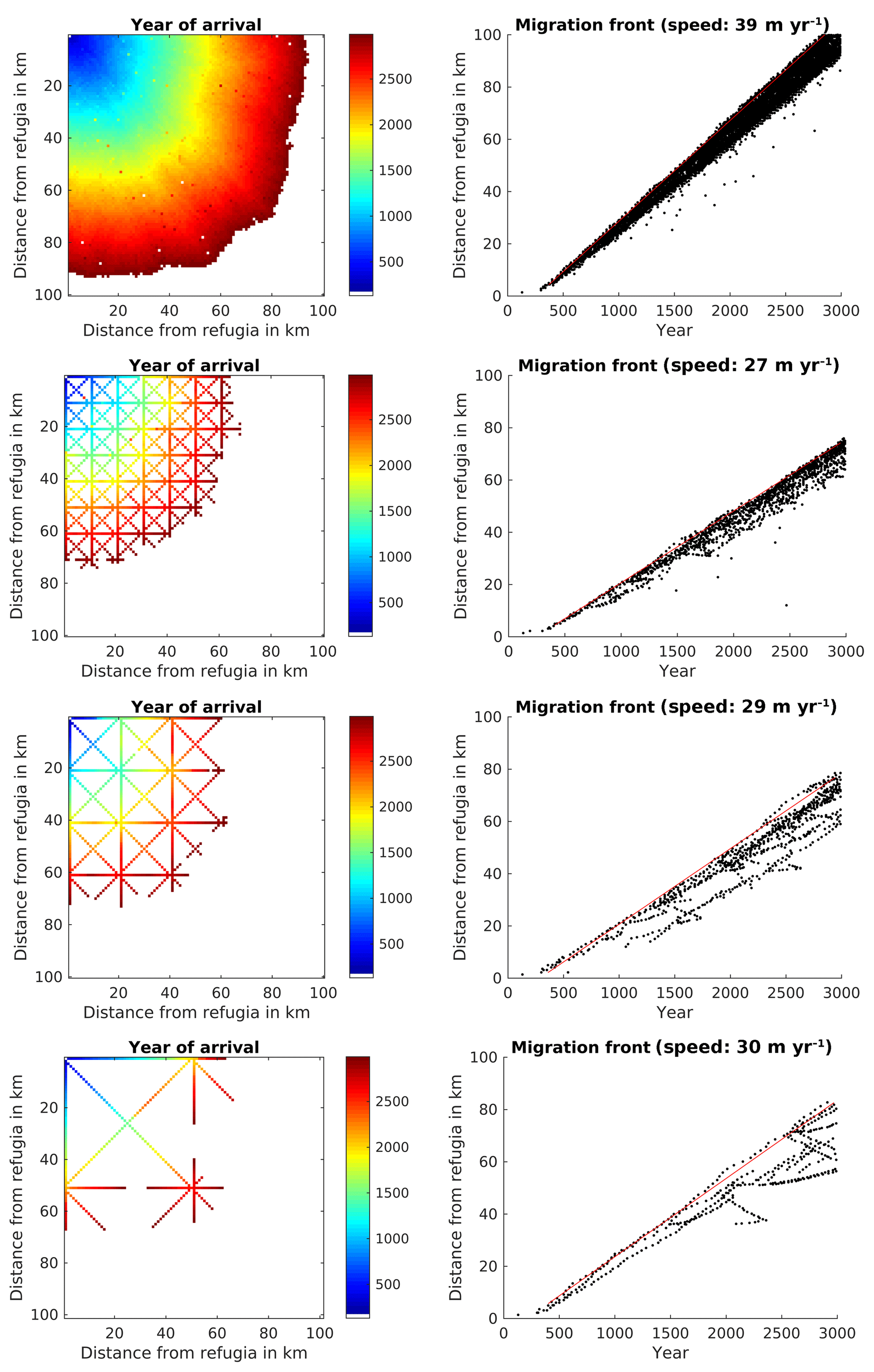
Figure 5Spread of Fagus sylvatica using the SMSM through an area of 100×100 grid cells with identical climate, using the full area (upper row of panels) or corridors every 10th, 20th, or 50th cell. For more explanation see Fig. 3.
Similarly to the FFTM simulations, the migration speed was reduced for simulations with transects (see Table 1 for a summary). Also comparable to the FFTM-based seed dispersal computation, calculation time per grid cell in the whole area (range for which the seed dispersal is computed) was increased by 16 % by the simulation of dispersal, but reduced to 35 %, 19 %, and 11 % by using the corridors. The proportion of calculation time spent for simulating the seed dispersal is comparable to the proportion using the FFT; it was 16 %, 19 %, close to 23 %, and 32 % (see Table 1).
Since the SMSM allows for adjusting the probability depending on the seed transport permeability of the terrain, we also simulated the migration within a non-homogenous dispersal area. The results of this simulation are displayed in Fig. 6. The total computation time for this simulation was 46 000 CPU h for 6000 years.
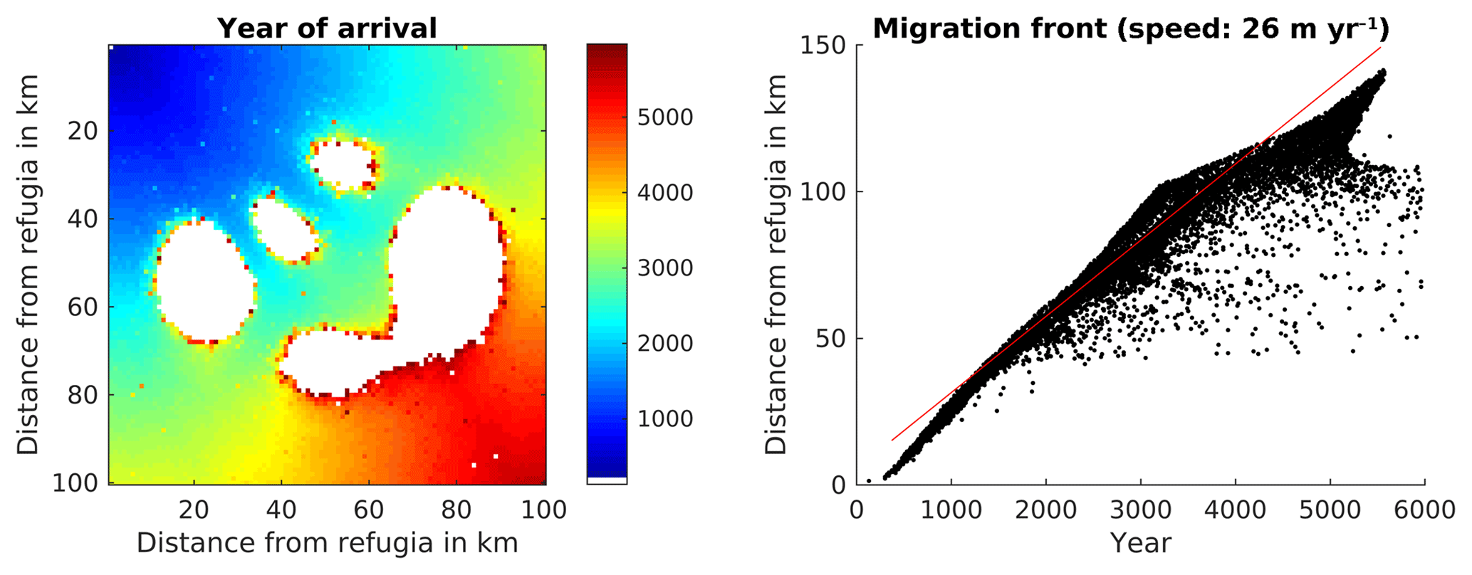
Figure 6Spread of Fagus sylvatica using the SMSM method through an area of 100×100 grid cells with identical climate but the probability of seed fall set to 0.00005 multiplied with the spatially explicit seed dispersal permeability value as shown in Fig. 2. Note that we increased the simulation time to 6000 years in order to have F. sylvatica establishing in all areas.
Though all cells of the virtual landscape had a similar climate, some cells were never occupied (see Fig. 6) because the seeds were not able to reach them due to the different permeability (which might not be reasonable for real-world simulations but demonstrates the method). Migration speed was different in different parts of the simulated area.
To our knowledge, in our study for the first time (tree) species migration has been implemented in a DGVM in a way that allows for simulations of simultaneously migrating and interacting species for large areas.
4.1 Performance of new migration methods
The presented new methods for simulating migration in DGVMs showed a promising performance in different aspects.
The first is the gain in efficiency with the FFTM and the SMSM methods compared to the traditional, straightforward approach of evaluating the seed transport from all cells to each other (Fig. S2.6 in Supplement S2). A two-dimensional FFT can be obtained by successive passes of the one-dimensional FFT, and hence the complexity will be the one-dimensional complexity squared (Gonzalez and Woods, 2002). The computational complexity for the FFTM is O(N2log 2(N)) for an N ×N grid discretizing the seed distribution, while the complexity of the direct implementation of the convolution approach in the SMSM is O(2KRN2) for an N ×N grid discretizing the seed distribution and R ×R kernel, with K being the number of iterations of the SMSM (for the derivation see Supplement S1). This can be computationally comparable to the FFTM for kernels with a short range of R. Secondly, simulating the local dynamics only along the corridors instead of in the full area resulted in a similar migration pattern, and the simulated migration speed was similar to that of the simulation with full grid cell cover (though it is slower, caused by the stochasticity of the establishment; see Table 1), but needed much less computing time (reduction of 88 % for the corridors every 50 km).
4.2 Comparison of the two dispersal methods
In this study we present two alternative methods for simulating dispersal, which differ in their properties. While the FFTM allows any type of seed dispersal kernel, the SMSM corresponds to a normal distribution kernel. Although other shapes of dispersal kernels can be approximated by weighted sums of normal distributions, each of which has to be simulated by an own SMSM, this will cause strong increases in computational demand. Additionally, the SMSM restricts the long tail of the distributions by the number of iterations, as the seeds can travel only one grid cell per iteration step.
On the other hand, the advantage of the SMSM lies in its ability (contrary to the FFTM) to modify the parameters of the seed dispersal kernel spatially, depending on the terrain. If instead of applying a single permeability for all directions, a different permeability is applied for each of the eight directions (e.g. north, northeast, east, etc.), this method also allows for a spatially explicit consideration of wind directions (which is not possible for the FFTM, as it relies on a universal kernel applied to the entire area). Hence, depending on the aim of the analysis, one algorithm or the other, or a combination of the algorithms, is most suitable.
While not implemented here, it should be theoretically possible to use the FFTM (preferably with corridors) for some homogenous parts of the simulated area and the SMSM for the remaining part in a single simulation. As long as the seed donor areas for both methods are exclusive, and the areas in which the seeds are allowed to disperse overlap at least the width of the kernel, we can see no reasons why this should not be feasible.
4.3 Comparison to other approaches
Our new species migration submodule FFTM uses for the first time an algorithm based on fast Fourier transform to simulate dispersal in a DGVM. Due to its efficiency, the FFT is one of the “workhorses” in mathematics, physics, and signal processing (Strang, 1994). In ecology, there have been a few applications using FFTs to simulate the dispersal of pollen (e.g. for risk analysis, Shaw et al., 2006; seeds, Pueyo et al., 2008; even in a course compendium, Powell, 2001), but not as a standard technique in DGVMs.
The SMSM, in turn, mimics the seed transport process itself in a simple and straightforward way, which to our knowledge has also not been implemented in DGVMs.
Both approaches are combined with features of modelling species migration that are already used in other dynamic vegetation models (see Snell, 2014).
The cellular automaton KISSMig (Nobis and Normand, 2014) simulates the spread of single species driven by a spatio-temporal grid of suitability and by transitions to the nearest-neighbour cells, which is similar to one iteration in the SMSM. The suitability-based models CATS (Dullinger et al., 2012) and MigClim (Engler and Guisan, 2009) simulate a simple demography of single species and spread explicitly based on a seed dispersal kernel.
To also account for ecophysiology, the CATS model was combined with LPJ-GUESS in a post-processing approach (Lehsten et al., 2014). A spatio-temporally explicit suitability for a single species was estimated from LPJ-GUESS simulations of the productivity of this species, assuming the presence of the other species. This suitability was subsequently used within CATS to simulate migration. Such a post-processing approach, however, does not include interactions among several migrating species.
Forest landscape models have been developed to integrate such feedbacks between species and dispersal (He et al., 2017; Shifley et al., 2017). These models simulate local vegetation dynamics with species interactions and dispersal by explicit calculation of seed or seedling transport probabilities with dispersal kernels of different shapes (e.g. LandClim, Schumacher et al., 2004, Landis, Mladenoff, 2004, Iland, Seidl et al., 2012). To capture spatial heterogeneity, they run at a comparably fine spatial resolution (about 20–100 m grid cells), allowing only for the simulation of relatively small areas due to computational demands.
To overcome such computational limits, several approaches for a spatial upscaling of the models have been put forward. For example, the forest landscape model TreeMig can operate at a coarser resolution (grid cell size 1000 m) because it aggregates within-stand heterogeneity by dynamic distributions and height classes (Lischke et al., 1998), which allows for applications at a larger scale, e.g. over all of Switzerland (Bugmann et al., 2014) or on a transect through Siberia (Epstein et al., 2007). Another upscaling of TreeMig was achieved by the D2C method (Nabel, 2015; Nabel and Lischke, 2013), which simulates local vegetation dynamics only in a subset of cells that are dynamically determined as representative for classes of similar cells. This method led to a computing time reduction of 30 %–85 % compared to the full simulation. This reduction is in a similar range for our transect method depending on the configuration of the corridors.
In DGVMs, the discretization problem resulting from the need to upscale from the fine scale at which migration processes act to the scale at which DGVMs work is very pronounced because they are designed to operate over very large extents (continents or the entire globe). Given the computational demands of the simulations, they are therefore typically running at a coarse resolution, for example 0.5 or 0.1∘ longitude–latitude, and simulate the vegetation dynamics at the centre of each of these grid cells, assuming this point to be representative for the entire cell.
Snell (2014) approached the discretization problem for the DGVM LPJ-GUESS by assuming that the numerous replicates of the vegetation dynamics on a patch are randomly distributed over the area of the grid cell (using 400 patches). Migration within the grid cell is treated similarly to an infection process, whereby the probability of a patch becoming infected (e.g. of the migrating species being able to establish) depends only on the number of already invaded patches within the grid cell. Only once a migrating species has managed to establish in a certain proportion of the patches of the simulated grid cell is further dispersal (explicit via a dispersal kernel) into surrounding grid cells possible. Yet, there is no spatial orientation of the patches within the grid cell and all simulations in this approach are strongly resolution dependent. Simulations of large areas such as continents remain computational challenging with this approach.
Our transect approach, similarly to the approach of Snell (2014), uses smaller representative spatial units of 1 km cells for a spatial upscaling. Since these small grid cells are arranged in contiguous corridors, the migration along these corridors can be simulated without or with only a small discretization error. The results indicate that the error potentially introduced by the interpolation to the rest of the area is also small.
The two approaches that we present differ in their ability to simulate heterogeneous landscapes (in terms of permeability). We suggest using the FFTM with corridors in homogenous landscapes (to speed up the computation) and using the SMSM without corridors in heterogeneous landscapes. In cases in which parts of the domain are heterogeneous (e.g. the regions around a mountainous area) and others are homogenous (e.g. lowlands), the cells can be arranged in a way that they cover the whole area in the heterogeneous part and only corridors in the homogenous part. In this setting the SMSM can still be used for the whole domain and an improvement of computation time can be achieved by only simulating the local vegetation dynamics in the homogenous parts of the domain. Thus, with our approaches, we have combined several advantages of the before-mentioned approaches: the seed dispersal from forest landscape models, improved by the novel FFTM or SMSM and the ecophysiology, and the structure and community dynamics of LPJ-GUESS. We furthermore found a compromise between discretization and efficiency by using the corridor method.
4.4 Potential further improvements
Despite the satisfying performance of the new methods in these first tests, some aspects require further development.
4.4.1 Computation time
Even with the computing time reduction by the corridor approach using a corridor distance of 50 km, the computing time required for the simulations including dispersal was still considerable. The reason is that the number of cells on the corridors (where the local dynamics are simulated) is larger than the number of replicates usually used in all the 1 or 0.5∘ grid cells simulated in traditional DGVMs. For large-scale applications, the approach should be further optimized, e.g. by choosing corridors even further apart from each other in homogenous areas and adapting the corridor density to the large-scale (between-grid-cell) heterogeneity of the terrain. The within-grid-cell heterogeneity in turn can be accounted for by deriving seed dispersal permeability that can be used in the SMSM approach. Another area of improvement lies in the technical implementation of the seed dispersal algorithm. In the current implementation, seed dispersal is performed at a single CPU, while all other CPUs wait until they receive the seeds. There are certainly ways to perform the seed dispersal computation on several nodes to decrease the waiting time. Furthermore, in multispecies simulations the dispersal has to be calculated for each migrating species. In this case, the dispersal of different species should be calculated on separate nodes. Enlarging simulation areas generally resulted in longer runtimes for all methods. Sometimes, however, the runtimes decreased in a pronounced way for the FFTM (Supplement S2). A cause for these decreases is that the efficiency of the FFT depends on possible factorizations of the domain size (Bronstein et al., 1995). For example, it is most efficient for domain sizes of 2n. Thus, a careful choice of the domain size or of an FFT code doing that automatically promises to speed up the FFTM. Figure S2.6 in Supplement S2 does not represent the differences in computation time between SMSM and FFTM as they are measured on the computing cluster when performing the actual simulation. While in Table 1 there was only a marginal difference between the calculations of the two methods, the differences in the MATLAB® implementation presented in Supplement S2 are up to an order of magnitude. It seems that MATLAB® uses a different optimization for calculating the fast Fourier transform even though both MATLAB® and the FFT libraries used on the computing cluster are based on the libraries provided by http://fftw.org (last access: 4 March 2019).
4.4.2 Migration speed reduction by corridor approach
It is to be expected that any sub-cell assumption results in discretization errors. In our case the assumption of a corridor reduced the migration speed. This needs to be taken into account when evaluating the result of such studies. The design of the corridors might also not have been optimal; a corridor wider than a single cell might result in less of a decrease in migration speed. However, these types of analysis are outside the scope of this study. One other aspect of using the corridors is that while a late successional species (in our case F. sylvatica) certainly has no problems to establish below the early successional species, in the case of an early successional species (e.g. B. pendula) migrating into an area occupied by a late successional species, the corridors might decrease the migration speed even more. An early successional species can only establish after sufficient light reaches the ground, either due to the senescence of a tree from the established species or a disturbance event. The narrow corridors might have strongly limited the availability of such grid cells. However, since early successional species typically have a good dispersal ability, this should not influence simulations of tree migration following climate change (e.g. after the last glaciation).
4.4.3 Parameterization of dispersal kernels and other plant parameters
In this study the focus was on developing and testing novel methods; i.e. we did not attempt to correctly simulate the spread of F. sylvatica over a defined time period. The calculated spread rates were well below most of the spread rates in the literature. F. sylvatica has been estimated to migrate with ca. 100 m per year based on pollen analyses by Bradshaw and Lindbladh (2005). Although such estimated high migration speeds could also be the result of glacial refugia located further north than assumed (Feurdean et al., 2013), our estimated migration speeds of 20–30 m yr−1 still seem rather low. However, in this paper we aimed to implement tree migration by using the parameterization of TreeMig in a DGVM and thereby allow for large-scale simulations. Our estimated migration rates of 20–30 m yr−1 are very close to the migration rates estimated for this parameterization for TreeMig by Meier et al. (2012), who estimated a value of 22 m yr−1. Hence, though we implemented the migration module into a conceptually very different model, the resulting migration rate remained relatively similar.
To perform model runs estimating the migration speed of any species would require a fine tuning of the age of maturity, seed production, dispersal parameters, germination rates, and seed survival (which are very rough estimates in TreeMig; Lischke et al., 2006) to generate the observed migration e.g. by comparing to migration rates based on pollen records. Unfortunately, though all of these parameters are most likely strongly influencing migration rates, they are not only hard to find in a study performed with similar methods for all tree species, but they are also likely to be highly variable depending on growth conditions and even the provenance of the individual tree. However, for a large-scale application at least the sensitivity of these parameters should be evaluated.
In our model, we assumed seed production to start at a fixed, species-specific height of maturity, which accounts for a developmental threshold but also growth and thus environmental conditions (similar to TreeMig, Lischke et al., 2006). Other studies used age of maturity as a trigger to start seed production, which has been shown to be important in determining tree migration rates (e.g. Nathan et al., 2011). The aim of this study was not a full sensitivity analysis but a study showing that a similar approach to that of Lischke et al. (2006) results in comparable migration rates. We will implement the option to use age of maturity in the next version of LPJ-GM.
Applications of our approach to simulate migration in the future are only suitable if the migration speed of any species is substantially faster than the migration speed that we reach for F. sylvatica (due to the time the period for which climate projections are available). Furthermore, independent of the model used, migration simulations are only suitable if the species are not typically planted, as in many commercial forests.
4.5 Potential for applications
The test simulations were performed on a virtual landscape of 100 km × 100 km, but eventually the method is aimed to allow for large-scale simulations over several millennia. Regarding memory requirements, this is possible with currently available hardware: test runs with landscapes of 4000 × 4000 grid cells (i.e. the size of Europe) were performed without technical problems, at least regarding the memory requirement (given 62 GB of RAM). The considerable computational cost, however, requires a relatively high amount of computing time, which might be reduced by efforts to speed up (due to efficient parallelization) the FFTM (currently the FFTM is performed on a single node, while the remaining nodes are idle; one could use all nodes to perform the FFTM) or by even further apart corridors.
The presented novel approaches offer high potential to simulate the spatio-temporal dynamics of species which are migrating and interacting with each other simultaneously. The approaches are not restricted to LPJ-GUESS, but can in principle be applied to other DGVMs or FLMs which simulate seed (or seedling) production and explicit regeneration. The presented methods need to be improved in terms of computing performance to allow for simulations of tree migration at continental scale and over paleo-timescales. Our study also shows that estimates for seed dispersal kernels for the major tree species need to be revised to allow for simulations of forest development, for example, over the Holocene.
The data behind all figures as well as the code for Supplement S2 are published on the DataGURU server (http://dataguru.lu.se, last access: 4 March 2019; https://doi.org/10.18161/migration_lehsten_2018, Lehsten et al., 2019a; https://doi.org/10.18161/seed_disp_code_2018, Lehsten et al., 2019b).
The Supplement contains a derivation of the variance of the seed dispersal kernel for the SMSM (Supplement S1) and an example evaluation of computation time difference between FFTM and the traditional method (Supplement S2). In this Supplement, an example code for the FFTM is given, together with code demonstrating the required transformation of the seed kernel for the FFTM, and an example calculation of the SMSM (Supplement S3). Species-specific parameters within the simulation are also given (Supplement S4). The supplement related to this article is available online at: https://doi.org/10.5194/gmd-12-893-2019-supplement.
VL, DL, and HL designed the study, and VL performed the simulations and the statistical analysis. MM and EL contributed to the study design, and MM also performed large parts of the coding. EL developed the formal proof in Supplement S1 and the computation-performance-related estimates in the Conclusion. All authors contributed to the writing of the paper.
The authors declare that they have no conflict of interest.
This study was funded by the Swiss National Science Foundation project
CompMig, no. 205321_163223.
Edited by:
Christoph Müller
Reviewed by: Julia Nabel and two anonymous
referees
Bradshaw, R. H. W. and Lindbladh, M.: Regional spread and stand-scale establishment of Fagus sylvatica and Picea abies in Scandinavia, Ecology, 86, 1679–1686, https://doi.org/10.1890/03-0785, 2005.
Bronstein, I. N., Semendjajew, K. A., Musiol, C., and Mühlig, H.: Taschenbuch der Mathematik, Verlag Harri Deutsch, Frankfurt am Main, 1995.
Bugmann, H. K. M., Brang, P., Elkin, C., Henne, P., Jakoby, O., Lévesque, M., Lischke, H., Psomas, A., Rigling, A., Wermelinger, B., and Zimmermann, N. E.: Climate change impacts on tree species, forest properties, and ecosystem services, in: CH2014-Impacts (2014): Toward Quantitative Scenarios of Climate Change Impacts in Switzerland, edited by: Foen, O., Meteoswiss, 2014.
Clarke, L., Glendinning, I., and Hempel, R.: The MPI Message Passing Interface Standard, in: Programming Environments for Massively Parallel Distributed Systems, edited by: Decker, R. R. and Birkhäuser, K. M., Basel, 1994.
Cooley, J. W. and Tukey, J. W.: An Algorithm for the Machine Calculation of Complex Fourier Series Mathematics of Computation An Algorithm for the Machine Calculation of Complex Fourier Series, Source, Math. Comput., 19, 297–301, https://doi.org/10.2307/2003354, 1965.
Dullinger, S., Willner, W., Plutzar, C., Englisch, T., Schratt-Ehrendorfer, L., Moser, D., Ertl, S., Essl, F., and Niklfeld, H.: Post-glacial migration lag restricts range filling of plants in the European Alps, Global Ecol. Biogeogr., 21, 829–840, https://doi.org/10.1111/j.1466-8238.2011.00732.x, 2012.
Engler, R. and Guisan, A.: MigClim: Predicting plant distribution and dispersal in a changing climate, Divers. Distrib., 15, 590–601, https://doi.org/10.1111/j.1472-4642.2009.00566.x, 2009.
Epstein, H. E., Yu, Q. Y. Q., Kaplan, J. O., and Lischke, H.: Simulating Future Changes in Arctic and Subarctic Vegetation, Comput. Sci. Eng., 9, 12–23, https://doi.org/10.1109/MCSE.2007.84, 2007.
Feurdean, A., Bhagwat, S. A., Willis, K. J., Birks, H. J. B., Lischke, H., and Hickler, T.: Tree Migration-Rates: Narrowing the Gap between Inferred Post-Glacial Rates and Projected Rates, PLoS One, 8, e71797, https://doi.org/10.1371/journal.pone.0071797, 2013.
Foley, J. A., Levis, S., Prentice, I. C., Pollard, D. and Thompson, S. L.: Coupling dynamic models of climate and vegetation, Glob. Change Biol., 4, 561–579, https://doi.org/10.1046/j.1365-2486.1998.00168.x, 1998.
Gonzalez, R. C. and Woods, R. E.: Digital Image Processing, 2nd Edn., Prentice Hall, 2002.
He, H. S., Gustafson, E. J., and Lischke, H.: Modeling forest landscapes in a changing climate: theory and application, Landscape Ecol., 32, 1299–1305, https://doi.org/10.1007/s10980-017-0529-4, 2017.
Hickler, T., Vohland, K., Feehan, J., Miller, P. A., Smith, B., Costa, L., Giesecke, T., Fronzek, S., Carter, T. R., Cramer, W., Kühn, I., and Sykes, M. T.: Projecting the future distribution of European potential natural vegetation zones with a generalized, tree species-based dynamic vegetation model, Global Ecol. Biogeogr., 21, 50–63, https://doi.org/10.1111/j.1466-8238.2010.00613.x, 2012.
Kruse, S., Gerdes, A., Kath, N. J., and Herzschuh, U.: Implementing spatially explicit wind-driven seed and pollen dispersal in the individual-based larch simulation model: LAVESI-WIND 1.0, Geosci. Model Dev., 11, 4451–4467, https://doi.org/10.5194/gmd-11-4451-2018, 2018.
Lehsten, D., Dullinger, S., Huber, K., Schurgers, G., Cheddadi, R., Laborde, H., Lehsten, V., Francois, L., Dury, M., and Sykes, M. T.: Modelling the Holocene migrational dynamics of Fagus sylvatica L. and Picea abies (L.) H. Karst, Global Ecol. Biogeogr., 23, 658–668, https://doi.org/10.1111/geb.12145, 2014.
Lehsten, V., Sykes, M. T., Scott, A. V., Tzanopoulos, J., Kallimanis, A., Mazaris, A., Verburg, P. H., Schulp, C. J. E., Potts, S. G., and Vogiatzakis, I.: Disentangling the effects of land-use change, climate and CO2 on projected future European habitat types, Global Ecol. Biogeogr., 24, 653–663, https://doi.org/10.1111/geb.12291, 2015.
Lehsten, V., Arneth, A., Spessa, A., Thonicke, K., and Moustakas, A.: The effect of fire on tree-grass coexistence in savannas: A simulation study, Int. J. Wildland Fire, 25, 137–146, https://doi.org/10.1071/WF14205, 2016.
Lehsten, L., Mischurow, M., Lindström, E., Lehsten, D., and Lischke, H.: Tree migration in virtual landscape, https://doi.org/10.18161/migration_lehsten_2018, 2019a.
Lehsten, L., Mischurow, M., Lindström, E., Lehsten, D., and Lischke, H.: Matlab code for supplementary material for Lehsten et al. GMD 2019, https://doi.org/10.18161/seed_disp_code_2018, 2019b.
Lindeskog, M., Arneth, A., Bondeau, A., Waha, K., Seaquist, J., Olin, S., and Smith, B.: Implications of accounting for land use in simulations of ecosystem carbon cycling in Africa, Earth Syst. Dynam., 4, 385–407, https://doi.org/10.5194/esd-4-385-2013, 2013.
Lischke, H., Löffler, T. J. and Fischlin, A.: Aggregation of individual trees and patches in forest succession models: Capturing variability with height structured, random, spatial distributions, Theor. Popul. Biol., 54, 213–226, https://doi.org/10.1006/tpbi.1998.1378, 1998.
Lischke, H., Zimmermann, N. E., Bolliger, J., Rickebusch, S., and Löffler, T. J.: TreeMig: A forest-landscape model for simulating spatio-temporal patterns from stand to landscape scale, Ecol. Model., 199, 409–420, https://doi.org/10.1016/j.ecolmodel.2005.11.046, 2006.
Meier, E. S., Lischke, H., Schmatz, D. R., and Zimmermann, N. E.: Climate, competition and connectivity affect future migration and ranges of European trees, Global Ecol. Biogeogr., 21, 164–178, https://doi.org/10.1111/j.1466-8238.2011.00669.x, 2012.
Mladenoff, D. J.: LANDIS and forest landscape models, Ecol. Model., 180, 7–19, https://doi.org/10.1016/j.ecolmodel.2004.03.016, 2004.
Nabel, J. E. M. S.: Upscaling with the dynamic two-layer classification concept (D2C): TreeMig-2L, an efficient implementation of the forest-landscape model TreeMig, Geosci. Model Dev., 8, 3563–3577, https://doi.org/10.5194/gmd-8-3563-2015, 2015.
Nabel, J. E. M. S. and Lischke, H.: Upscaling of spatially explicit and linked time- and space-discrete models simulating vegetation dynamics under climate change, in: 27th International Conference on Environmental Informatics for Environmental Protection, Sustainable Development and Risk Management, EnviroInfo 2013, edited by: Page, B., Göbel, F. A. G. J., and Wohlgemuth, V., Hamburg, 842–850, 2013.
Nathan, R., Horvitz, N., He, Y., Kuparinen, A., Schurr, F. M., and Katul, G. G.: Spread of North American wind-dispersed trees in future environments, Ecol. Lett., 14, 211–219, https://doi.org/10.1111/j.1461-0248.2010.01573.x, 2011.
Neilson, R. P., Pitelka, L. F., Solomon, A. M., Nathan, R., Midgley, G. F., Fragoso, J. M. V., Lischke, H., and Thompson, K.: Forecasting regional to global plant migration in response to climate change, Bioscience, 55, 749–759, 2005.
Nobis, M. P. and Normand, S.: KISSMig – a simple model for R to account for limited migration in analyses of species distributions, Ecography, 37, 1282–1287, https://doi.org/10.1111/ecog.00930, 2014.
Powell, J.: Spatiotemporal models in ecology; an introduction to integro- difference equations, Utah State University, available at: http://www.math.usu.edu/powell/wauclass/labs.pdf (last access: 4 March 2019), 2001.
Pueyo, Y., Kefi, S., Alados, C. L., and Rietkerk, M.: Dispersal strategies and spatial organization of vegetation in arid ecosystems, Oikos, 117, 1522–1532, https://doi.org/10.1111/j.0030-1299.2008.16735.x, 2008.
Quillet, A., Peng, C., and Garneau, M.: Toward dynamic global vegetation models for simulating vegetation–climate interactions and feedbacks: recent developments, limitations, and future challenges, Environ. Rev., 18, 333–353, https://doi.org/10.1139/A10-016, 2010.
Sato, H. and Ise, T.: Effect of plant dynamic processes on African vegetation responses to climate change: Analysis using the spatially explicit individual-based dynamic global vegetation model (SEIB-DGVM), J. Geophys. Res., 117, G03017, https://doi.org/10.1029/2012JG002056, 2012.
Sato, H., Itoh, A., and Kohyama, T.: SEIB–DGVM: A new Dynamic Global Vegetation Model using a spatially explicit individual-based approach, Ecol. Model., 200, 279–307, https://doi.org/10.1016/j.ecolmodel.2006.09.006, 2007.
Scherstjanoi, M., Kaplan, J. O., and Lischke, H.: Application of a computationally efficient method to approximate gap model results with a probabilistic approach, Geosci. Model Dev., 7, 1543–1571, https://doi.org/10.5194/gmd-7-1543-2014, 2014.
Schumacher, S., Bugmann, H., and Mladenoff, D. J.: Improving the formulation of tree growth and succession in a spatially explicit landscape model, Ecol. Model., 180, 175–194, https://doi.org/10.1016/j.ecolmodel.2003.12.055, 2004.
Seidl, R., Rammer, W., Scheller, R. M., and Spies, T. A.: An individual-based process model to simulate landscape-scale forest ecosystem dynamics, Ecol. Model., 231, 87–100, https://doi.org/10.1016/j.ecolmodel.2012.02.015, 2012.
Shaw, M. W., Harwood, T. D., Wilkinson, M. J., and Elliott, L.: Assembling spatially explicit landscape models of pollen and spore dispersal by wind for risk assessment, P. Roy. Soc. B Biol. Sci., 273, 1705–1713, https://doi.org/10.1098/rspb.2006.3491, 2006.
Shifley, S. R., He, H. S., Lischke, H., Wang, W. J., Jin, W., Gustafson, E. J., Thompson, J. R., Thompson, F. R., Dijak, W. D., and Yang, J.: The past and future of modeling forest dynamics: from growth and yield curves to forest landscape models, Landscape Ecol., 32, 1307–1325, https://doi.org/10.1007/s10980-017-0540-9, 2017.
Shiryaev, A. N.: Probability, 3rd Edn., Springer Verlag, New York, 2016.
Sitch, S., Smith, B., Prentice, I. C., Arneth, A., Bondeau, A., Cramer, W., Kaplan, J. O., Levis, S., Lucht, W., Sykes, M. T., Thonicke, K., and Venevsky, S.: Evaluation of ecosystem dynamics, plant geography and terrestrial carbon cycling in the LPJ dynamic global vegetation model, Glob. Change Biol., 9, 161–185, 2003.
Smith, B., Prentice, I. C., and Sykes, M. T.: Representation of vegetation dynamics in the modelling of terrestrial ecosystems: comparing two contrasting approaches within European climate space, Global Ecol. Biogeogr., 10, 621–637, 2001.
Smith, B., Wårlind, D., Arneth, A., Hickler, T., Leadley, P., Siltberg, J., and Zaehle, S.: Implications of incorporating N cycling and N limitations on primary production in an individual-based dynamic vegetation model, Biogeosciences, 11, 2027–2054, https://doi.org/10.5194/bg-11-2027-2014, 2014.
Snell, R. S.: Simulating long-distance seed dispersal in a dynamic vegetation model, Global Ecol. Biogeogr., 23, 89–98, https://doi.org/10.1111/geb.12106, 2014.
Snell, R. S., Huth, A., Nabel, J. E. M. S., Bocedi, G., Travis, J. M. J., Gravel, D., Bugmann, H., Gutiérrez, A. G., Hickler, T., Higgins, S. I., Reineking, B., Scherstjanoi, M., Zurbriggen, N., and Lischke, H.: Using dynamic vegetation models to simulate plant range shifts, Ecography, 37, 1184–1197, https://doi.org/10.1111/ecog.00580, 2014.
Strang, G.: Wavelets, Am. Sci., 82, 250–255, 1994.
Yue, C., Ciais, P., Luyssaert, S., Li, W., McGrath, M. J., Chang, J., and Peng, S.: Representing anthropogenic gross land use change, wood harvest, and forest age dynamics in a global vegetation model ORCHIDEE-MICT v8.4.2, Geosci. Model Dev., 11, 409–428, https://doi.org/10.5194/gmd-11-409-2018, 2018.