the Creative Commons Attribution 4.0 License.
the Creative Commons Attribution 4.0 License.
 | 08 Mar 2019
The Open Global Glacier Model (OGGM) v1.1
Fabien Maussion
Anton Butenko
Nicolas Champollion
Matthias Dusch
Julia Eis
Kévin Fourteau
Philipp Gregor
Alexander H. Jarosch
Johannes Landmann
Felix Oesterle
Beatriz Recinos
Timo Rothenpieler
Anouk Vlug
Christian T. Wild
Ben Marzeion
Despite their importance for sea-level rise, seasonal water availability, and as a source of geohazards, mountain glaciers are one of the few remaining subsystems of the global climate system for which no globally applicable, open source, community-driven model exists. Here we present the Open Global Glacier Model (OGGM), developed to provide a modular and open-source numerical model framework for simulating past and future change of any glacier in the world. The modeling chain comprises data downloading tools (glacier outlines, topography, climate, validation data), a preprocessing module, a mass-balance model, a distributed ice thickness estimation model, and an ice-flow model. The monthly mass balance is obtained from gridded climate data and a temperature index melt model. To our knowledge, OGGM is the first global model to explicitly simulate glacier dynamics: the model relies on the shallow-ice approximation to compute the depth-integrated flux of ice along multiple connected flow lines. In this paper, we describe and illustrate each processing step by applying the model to a selection of glaciers before running global simulations under idealized climate forcings. Even without an in-depth calibration, the model shows very realistic behavior. We are able to reproduce earlier estimates of global glacier volume by varying the ice dynamical parameters within a range of plausible values. At the same time, the increased complexity of OGGM compared to other prevalent global glacier models comes at a reasonable computational cost: several dozen glaciers can be simulated on a personal computer, whereas global simulations realized in a supercomputing environment take up to a few hours per century. Thanks to the modular framework, modules of various complexity can be added to the code base, which allows for new kinds of model intercomparison studies in a controlled environment. Future developments will add new physical processes to the model as well as automated calibration tools. Extensions or alternative parameterizations can be easily added by the community thanks to comprehensive documentation. OGGM spans a wide range of applications, from ice–climate interaction studies at millennial timescales to estimates of the contribution of glaciers to past and future sea-level change. It has the potential to become a self-sustained community-driven model for global and regional glacier evolution.


Glaciers constitute natural low-pass filters of atmospheric variability. They allow people to directly perceive slow changes of the climate system, which would otherwise be masked by short-term noise in human perception. As glaciers form prominent features of many landscapes, shrinking glaciers have become an icon of climate change.
However, impacts of glacier change – whether growth or shrinkage – go far beyond this sentimental aspect: glaciers are important regulators of water availability in many regions of the world (Kaser et al., 2010; Huss, 2011; Immerzeel et al., 2012), and retreating glaciers can lead to increased geohazards (see Richardson and Reynolds, 2000, for an overview). Even though the ice mass stored in glaciers is small compared to the Greenland and Antarctic ice sheets (<1 %), glacier melt has contributed significantly to past sea-level rise (SLR; e.g., Cogley, 2009; Leclercq et al., 2011; Marzeion et al., 2012b; Gardner et al., 2013). Glaciers have probably been the biggest single source of observed SLR since 1900 and will continue to be a major source of SLR in the 21st century (e.g., Church et al., 2013; Gregory et al., 2013).
Therefore, it is a pressing task to improve the knowledge of how glaciers change when subjected to climate change, both natural and anthropogenic (Marzeion et al., 2014a). The main obstacle to achieving progress in this respect is a severe undersampling problem: direct glaciological measurements of mass balances have been performed on ∼ 300 glaciers world wide (≈ 0.1 % of all glaciers on Earth). The number of glaciers on which these types of measurements have been carried out for time periods longer than 30 years, i.e., over periods that potentially allow for the detection of a climate change signal, is one order of magnitude smaller (Zemp et al., 2009). Length variations of glaciers have been observed for substantially longer periods of time (Oerlemans, 1994, 2005). These variations are, however, much more difficult to understand, as large glacier length fluctuations may arise from intrinsic climate variability (Roe and O'Neal, 2009; Roe, 2011). Data obtained by remote sensing allow for gravimetric assessments of ice mass change or volume change estimates obtained by differencing digital elevation models (DEMs). Unfortunately, they are only available for the past decade (e.g., Gardner et al., 2013).
During the past few years, great progress has been made in methods to model glaciers globally (Radić and Hock, 2011, 2014; Giesen and Oerlemans, 2012, 2013; Marzeion et al., 2012a, b, 2014a, b; Huss and Hock, 2015). While these approaches yield consistent results at the global scale, all of them suffer from greater uncertainties at the regional and local scales. These uncertainties stem from the great level of abstraction of the key processes (Marzeion et al., 2012b, 2014b), from the need to spatially interpolate model parameters (Radić and Hock, 2011, 2014; Giesen and Oerlemans, 2012, 2013), and from uncertainties in the boundary and initial conditions. All models lack ice dynamics, most lack frontal ablation (with the exception of Huss and Hock, 2015), and all lack modulation of the surface mass balance by debris cover and snow redistribution (wind and avalanches). Only one model (Marzeion et al., 2012b) was able to provide estimates of past glacier volume changes for the 20th century. None of these models are open-source.
Mountain glaciers are one of the few remaining subsystems of the global climate system for which no globally applicable, open-source, community-driven model exists. The ice sheet modeling community is a better exemplar, with models such as the Parallel Ice Sheet Model (Winkelmann et al., 2011), Elmer/Ice (http://elmerice.elmerfem.org/, last access: 27 February 2019), Glimmer-CISM (https://csdms.colorado.edu/wiki/Model:Glimmer-CISM, last access: 27 February 2019), or ISSM (https://issm.jpl.nasa.gov/, last access: 27 February 2019). These models have been applied to mountain glaciers as well, but cannot be applied globally out-of-the-box. While the atmospheric modeling community has a long tradition of sharing models (e.g., the Weather Research and Forecasting model – WRF) or comparing them (e.g., the Coupled Model Intercomparison Project – CMIP), recent initiatives originating from the glaciological community show a new willingness to better coordinate global research efforts following the CMIP example (e.g., the Glacier Model Intercomparison Project1 or the Glacier Ice Thickness Estimation Working Group2).
In the recent past, great advances have been made in the global availability of data and methods relevant for glacier modeling, spanning glacier outlines (Pfeffer et al., 2014), automatized glacier centerline identification (e.g., Kienholz et al., 2014), bedrock inversion methods (e.g., Huss and Farinotti, 2012), and global topographic datasets (e.g., Farr et al., 2007). Taken together, these advances now allow the ice dynamics of glaciers to be simulated at the global scale, provided that adequate modeling platforms are available. In this paper, we present the Open Global Glacier Model (OGGM), developed to provide a modular and open-source numerical model framework for consistently simulating past and future global-scale glacier change.
Global not only in the sense of leading to meaningful results for all glaciers combined, but also for any small ensemble of glaciers, e.g., at the headwater catchment scale. Modular to allow different approaches to the representation of ice flow and surface mass balance to be combined and compared against one another. Open source so that the code can be read and used by anyone and so that new modules can be added and discussed by the community, following the principles of open governance. Consistent between past and future in order to provide uncertainty measures at all realizable scales.
This paper describes the basic structure and primordial assumptions of the model (as of version 1.1). We present the results of a series of single glacier and global simulations demonstrating the model's usage and potential. This will be followed by a description of the software requirements and the testing framework. Finally, we will discuss the potential for future developments that could be conducted by any interested research team.
The starting point of OGGM is the Randolph Glacier Inventory (RGI; RGI Consortium, 2017; Pfeffer et al., 2014), and our goal is to simulate the past and future evolution of all of the 216 502 inventoried glaciers worldwide (as of RGI V6). This “glacier-centric” approach is the one followed by most global and regional models to date; its advantages and disadvantages will be discussed in Sect. 3.6.4. Provided with the glacier outlines, and topographical and climate data at reasonable resolution and accuracy, the model should be able to (i) provide a local map of the glacier including topography and hypsometry, (ii) estimate the glacier's total ice volume and compute a map of the bedrock topography, (iii) compute the surface climatic mass balance and (if applicable) at its front via frontal ablation, (iv) simulate the glacier's dynamical evolution under various climate forcings, and (v) provide an estimate of the uncertainties associated with the modeling chain.
For each of these steps, several choices are possible regarding the input data to be used, the numerical solver, or the parameterizations to be applied. Any given choice is driven by subjective considerations about data availability, the estimated accuracy of boundary conditions (such as topography), and by technical considerations such as the computational resources available. In this paper we present one way to realize these steps using OGGM, which, in our opinion, is the best compromise between model complexity, data availability, and computational effort to date. However, the OGGM software is built in such a way that future improvements and new approaches can be implemented, tested, and applied at minimal cost by ourselves or a larger community.
2.1 Example workflow
We illustrate, using an example, how the OGGM workflow is applied to Tasman Glacier, New Zealand (Fig. 1). In the following we briefly describe the purpose of each processing step, and more details are provided in Sect. 3:
-
Preprocessing. The glacier outlines extracted from the RGI are projected onto a local gridded map of the glacier (Fig. 1a). Depending on the glacier's location, a suitable source for the topographical data is automatically downloaded (here SRTM) and interpolated to the local grid. The map's spatial resolution depends on the size of the glacier (here, 150 m).
-
Flow lines. The glacier centerlines are computed using a geometrical routing algorithm (adapted from Kienholz et al., 2014, Fig. 1b), filtered and slightly modified to become glacier flow lines with a fixed grid spacing.
-
Catchment areas and widths. The geometrical widths along the flow lines are obtained by intersecting the normals at each grid point with the glacier outlines and the tributaries' catchment areas (Fig. 1c). Each tributary and the main flow line has a catchment area, which is then used to correct the geometrical widths so that the flow-line representation of the glacier is in close accordance with the actual altitude–area distribution of the glacier (Fig. 1d, note that the normals are now corrected and centered).
-
Climate data and mass balance. Gridded climate data (monthly temperature and precipitation) are interpolated to the glacier location and temperature is corrected for altitude using a linear gradient. These climate time series are used to compute the glacier mass balance at each flow line's grid point for any month in the past.
-
Ice thickness inversion. Using the mass-balance data computed above and relying on mass-conservation considerations, an estimate of the ice flux along each glacier cross section can be computed. By making assumptions about the shape of the cross section (parabolic or rectangular) and using the physics of ice flow, the model computes the thickness of the glacier along the flow lines and the total volume of the glacier (Fig. 1e).
-
Glacier evolution. A dynamical flow-line model is used to simulate the advance and retreat of the glacier as a response of the surface mass-balance forcing. Here (Fig. 1f), a 100-year-long random climate sequence leads to a glacier advance.

Figure 1Example of the OGGM workflow applied to Tasman Glacier, New Zealand: (a) topographical data preprocessing; (b) computation of the flow lines; (c) geometrical glacier width determination (the colors indicate the different flow lines); (d) width correction according to catchment areas and altitude–area distribution (see Fig. 2 and main text for details); (e) ice thickness inversion; and (f) random 100-year-long glacier evolution run leading to a glacier advance. See Sect. 2.1 for details.
2.2 Model structure
The OGGM model is built around the notion of tasks, which have to be applied sequentially to single glacier or a set of glaciers. There are two types of tasks:
-
Entity tasks are tasks which are applied on single glaciers individually and do not require information from other glaciers (this encompasses the majority of the OGGM's tasks). Most often they need to be applied sequentially (for example, it is not possible to compute the centerlines without having read the topographical data first).
-
Global tasks are tasks that are run on a set of glaciers. This encompasses the calibration and validation routines, which need to gather data across a number of reference glaciers.
This model structure has several advantages: the same entity task can be run in parallel on several glaciers at the same time, and they allow a modular workflow. Indeed, a task can seamlessly be replaced by another similar task, as long as the required input and output formats are agreed upon beforehand. The output of each task is made persistent by storage on disk, allowing for later use by a subsequent task, even in a separate run or on another machine. For example, the preprocessing tasks store the topography data in a netCDF file, which is then read by the centerlines task, which itself writes its output in a vector file format.
In this paper we will refrain from naming the tasks by their function name in the code, as these are likely to change in the future and are sometimes organized in a non-trivial way as a result of implementation details. Therefore, the next section is called “Modules”, where each module can be seen as a collection of tasks developed towards a certain goal.
The modules are described in the order in which they are applied for a model run. When we provide a specific value for a model parameter in the text, we refer to the model's default parameter value; this value can be changed by the user at run time.
3.1 Preprocessing
The objective of the preprocessing module is to set up the geographical input data for each glacier (the glacier outlines and the local topography). First, a Cartesian local map projection is defined: we use a local Transverse Mercator projection centered on the glacier. Then, a suitable topographical data source is automatically chosen, depending on the glacier's location. Currently we use the following:
-
the Shuttle Radar Topography Mission (SRTM) 90 m Digital Elevation Database v4.1 (Jarvis et al., 2008) for all locations in the 60∘ S–60∘ N range (data acquisition: 2000);
-
the Greenland Mapping Project (GIMP) digital elevation model (Howat et al., 2014) for mountain glaciers in Greenland (data acquisition: 2003 to 2009);
-
the Radarsat Antarctic Mapping Project (RAMP) digital elevation model, version 2 (Liu et al., 2015) for mountain glaciers in Antarctica with the exception of some peripheral islands (data acquisition: 1940 to 1999); and
-
the Viewfinder Panoramas DEM3 product (http://viewfinderpanoramas.org/dem3.html, last access: 27 February 2019) elsewhere (most notably, North America, Russia, Iceland, and Svalbard)
All datasets have a comparable spatial resolution (from 30 to 90 m, or 3 arcsec). Using different data sources is problematic but unavoidable as there is no consistent, gap-free, globally available digital elevation model (DEM) to date. The Advanced Spaceborne Thermal Emission and Reflection Radiometer (ASTER) global digital elevation model version 2 (GDEM V2) is available globally but was quickly eliminated due to large data voids and artefacts, in particular in the Arctic. These artefacts are often tagged as valid data and cannot be easily detected automatically. The Viewfinder Panoramas products rely on the same sources but have been corrected manually (mostly with topographic maps; Jonathan de Ferranti, personal communication, 2017); thus, this ensures a more realistic void filling. Although they have nearly global coverage, the DEM3 products are not used in place of as it is not easy to retrieve the original data sources used to generate them (the information is scattered around the website, although ASTER and SRTM are the main data sources in most cases). It must be noted that a number of glaciers will still suffer from poor topographic information and/or a date of data acquisition which does not match that of the RGI outlines. Either the errors are large or obvious (in which case the model will not run), or they are left unnoticed. The importance of reliable topographic data for global glacier modeling will be the topic of a follow-up study.3
The spatial resolution of the target local grid depends on the size of the glacier. The default spatial resolution is to use a square relation to the glacier size (dx=aS½, with a=14 and S the area of the glacier in km2) clipped to a predefined minimum (10 m) and maximum (200 m) value. After the interpolation to the target grid, the topography is smoothed using a Gaussian filter with a radius of 250 m (this value does not change with the local glacier map resolution because it is meant to be applied to the original DEM, not the interpolated one). This smoothing is driven by practical considerations, as the model becomes unstable if the boundary conditions are too noisy (see also Bahr et al., 2014, for a discussion about the unavoidable trade-off between resolution and accuracy).
3.2 Flow lines and catchments
The glacier centerlines are computed following an algorithm developed by Kienholz et al. (2014) and adapted for our purposes. This algorithm was chosen because it allows one to compute multiple centerlines and to define a main branch fed by any number of tributaries. In general we found the method to be very robust, although some glaciers will obviously not have the optimal number of centerlines, with either too many (frequent in the case of large cirque glaciers) or too few (some tributary branches have no centerlines). However, these errors are assumed to play a relatively minor role compared to other uncertainties in the model chain.
In the model semantics, the original “centerlines” are then converted to “flow lines”: the points defining the line geometries are interpolated to be equidistant from one another (the default spacing along the line is twice that of the local glacier map, i.e., varying between 20 and 400 m depending on the glacier size), and the tail of the tributaries are cut before reaching their descendant (see the differences between Fig. 1b and c, or between Fig. 2a and b). Each grid point's elevation is obtained from the underlying topography. By construction, upslope trajectories or sinks along the flow line are rare; however, this can still occur when the glacier outlines are poorly defined or because of errors in the gridded topography. In these cases, we interpolate the heights (in the case of a deepening) or cut the first grid points of the line (in the case of an upslope trajectory starting from the flow-line's head) until only positive slopes larger than 1.5∘ remain. This is necessary because sinks along a flow line are incompatible with the forward dynamical model, which will fill them with ice and create undesirable spin-up issues.
The flow lines are then sorted according to their Strahler number (a measure of branching complexity defined by Strahler, 1952, and commonly used in hydrological applications), from the lowest (line without tributaries but with possible descendants) to the highest (the main – and longest – centerline). This order is important for the mass flow routing; each flow line contains a reference to its descendant, and this reference is used by the inversion and dynamical models to transfer mass from the tributaries towards the main flow line.
The width of each grid point along the flow line is computed in four steps. First, the catchment area of each flow line is computed using a routing algorithm similar to that used to compute the centerlines (Fig. 2a). Then the geometrical widths are computed by intersecting the flow-line's normal to the boundaries of either the individual catchments or the glacier itself (Fig. 2b). These geometrical widths are then corrected by a factor specific for each altitudinal bin (Fig. 2c), so that the true altitude area distribution of the glacier is approximately preserved (Fig. 2d). Finally, these widths are multiplied by a single factor ensuring that the total area of the glacier is the exact same as the one provided by the RGI, ensuring consistency with future model intercomparisons.
At this stage, it is important to note that the map representation of the flow-line glacier presented in Fig. 2c is purely artificial. The fact that the glacier cross sections are overlapping is irrelevant. The role of the flow lines is to represent the actual flow of ice as accurately as possible while conserving the fundamental aspects of the real glacier: slope, altitude, area, and geometry. The flow-line approximation will work better for valley glaciers (like Tasman Glacier shown above) than for cirque glaciers (such as the Upper Grindelwald glacier). For ice caps, the flow-line representation is likely to work poorly, as discussed in Sect. 3.6.2. From Fig. 2c one can see that future improvements of the mass-balance model based on, e.g., topographical shading or snow redistribution are made possible by knowledge about the flow-lines' location.
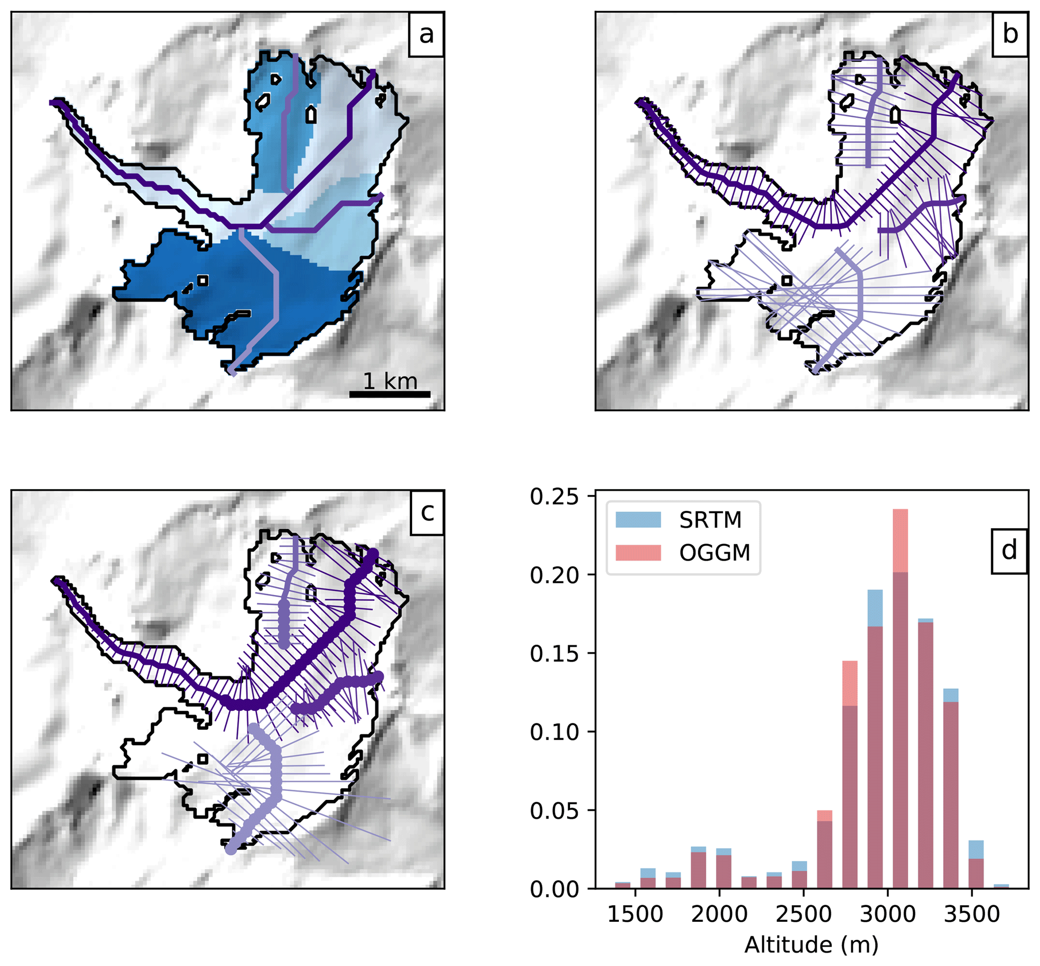
Figure 2Example of the flow-lines' width determination algorithm applied to the Upper Grindelwald glacier, Switzerland: (a) determination of each flow-line's catchment area; (b) geometrical widths; (c) widths corrected for the altitude–area distribution – the bold lines represent the grid points where the cross section touches a neighboring catchment; and (d) the frequency distribution of the glacier area per altitude bin, as represented by OGGM and by the SRTM topography.
3.3 Climate data and mass balance
The mass-balance model implemented in OGGM is an extended version of the temperature index melt model presented by Marzeion et al. (2012b). The monthly mass balance mi at an elevation z is computed as follows:
where is the monthly solid precipitation, pf is a global precipitation correction factor (defaults to 2.5, see Appendix A), μ* is the glacier's temperature sensitivity, Ti is the monthly air temperature, TMelt is the monthly air temperature above which ice melt is assumed to occur (default: −1 ∘C, chosen because melting days can occur even if the monthly average temperature is below 0 ∘C), and ε is a residual (or bias correction) term. Solid precipitation is computed as a fraction of the total precipitation: 100 % solid if (default: 0 ∘C); 0 % if Ti>=TLiquid (default: 2 ∘C); and linearly interpolated in between. The parameter μ* indicates the temperature sensitivity of the glacier and needs to be calibrated. For this paper, the temperature and precipitation time series (1901–2016) are obtained from gridded observations (CRU TS4.01; Harris et al., 2014, see Appendix A). The temperature lapse rate is set to a constant value (default: 6.5 K km−1) or it can be time-dependant and computed from a linear fit of the nine surrounding grid points.
For the calibration of the temperature sensitivity parameter μ* we use the method described by Marzeion et al. (2012b) and successfully applied many times since then (e.g., Marzeion et al., 2014a, 2015, 2018). Although the general procedure did not change, its peculiarity justifies describing it here. We will start by noting that μ* depends on many factors, most of them glacier-specific (e.g., avalanches, topographical shading, cloudiness), and others that are related to systematic biases in the input data (e.g., climate, topography). As a result, μ* can vary greatly between neighboring glaciers without obvious physical reasons. The calibration procedure implemented in OGGM makes use of these apparent handicaps by turning them into assets.
The procedure begins with glaciers for which we have direct observations of specific mass balance (N=254, see Appendix B). For each of these glaciers, annual sensitivities μ(t) are computed from Eq. (1) by requiring that the glacier specific mass balance is equal to zero.4 is the glacier integrated mass balance computed for a 31-year period centered around the year t and for a constant glacier geometry fixed at the RGI outline's date (e.g., 2003 in the Alps). The process is illustrated in Fig. 3c (blue line): around 1920 the climate was cold and wet (Fig. 3a and b), and as a consequence the hypothetical temperature sensitivity required to maintain the 2003 glacier geometry needs to be high. Inversely, the more recent climate is warmer and the temperature sensitivity needs to become smaller for the glacier to remain stable.
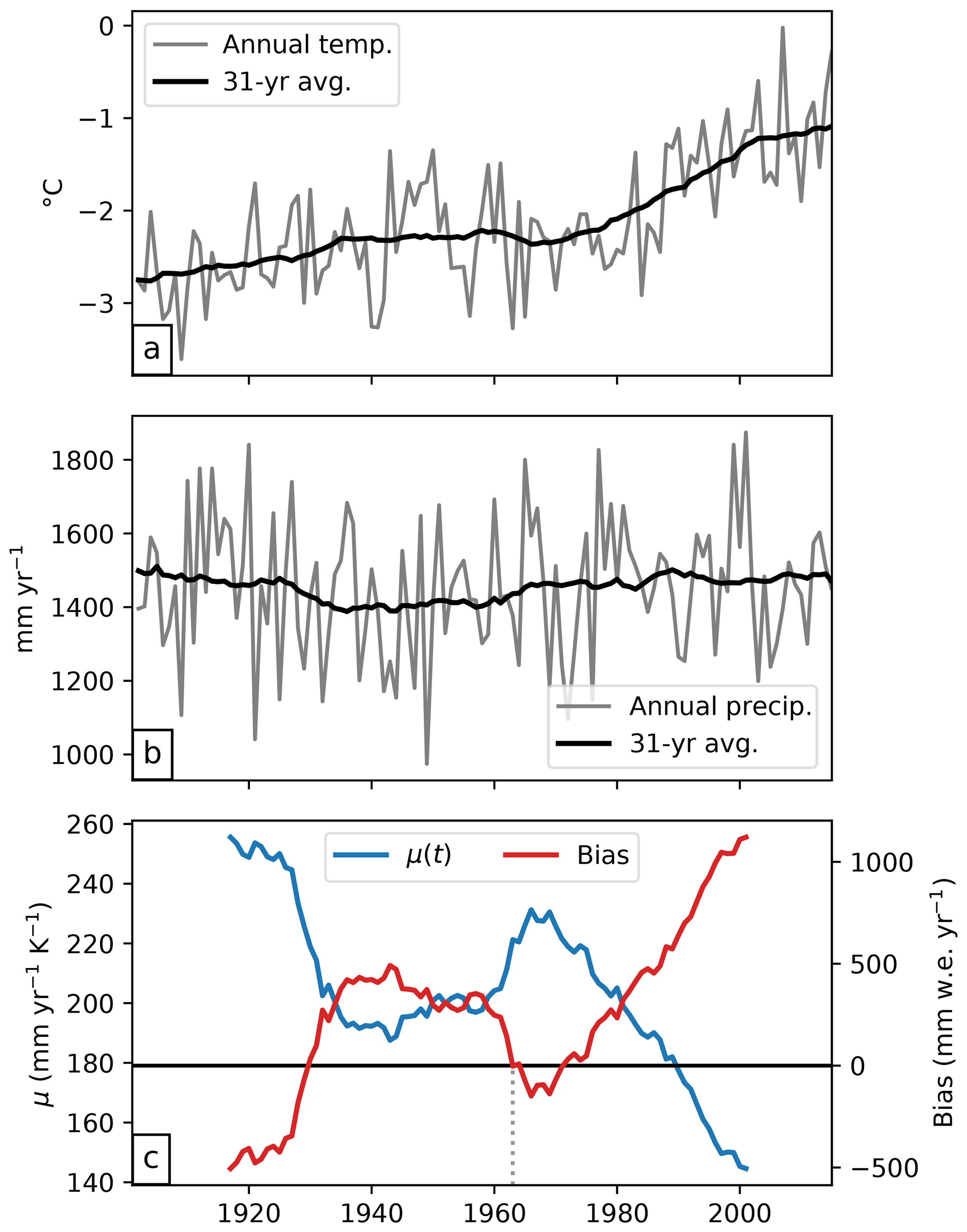
Figure 3Calibration procedure for μ* applied to the Hintereisferner Glacier, Austria. (a, b) Annual and 31-year average of temperature and precipitation obtained from the nearest CRU grid point (altitude 2700 m a.s.l.). (c) Time series of the μ candidates (mm yr−1 K−1) and their associated mass-balance bias (mm w.e. yr−1, right axis) in comparison to observations. The vertical dashed line marks the time where the bias is closest to zero (t*).
These hypothetical, time-dependent μ(t) are called “candidates”, as it is likely (but not certain) that at least one of them is the correct μ*. To determine which of the candidates is suitable, we then compute the mass-balance time series for each of the μ(t) and compute their bias ε with respect to observations (red line in Fig. 3c). Note that the period over which the observations are taken is not relevant for the bias computation, and each μ candidate can produce a mass balance for any year, as per Eq. (1). In comparison to observations, μ(t=2000) is too low and produces mass balances with a positive bias. Inversely, μ(t=1920) is too high and leads to a negative bias. For 3 years, the bias is close to or crossing the zero line and μ(t) is therefore very close to the ideal μ*. These dates represent the center of a 31-year-long climate period where today's glacier would be in equilibrium and maintain its current geometry. From these three candidates, we pick the date with the smallest bias and call it t*. This t* is an actual date but is mostly an abstract concept: we make use of it in the next step.
For the vast majority of the glaciers, μ* and t* are unknown. For these we could interpolate the μ* (probably the most obvious solution), or we could interpolate t*; indeed, the procedure above can be reversed and t* can be used to retrieve μ*, again by requiring that is equal to zero (Eq. 1). We interpolate t* to all glaciers without observations using inverse distance interpolation from the 10 closest locations (which can be quite far away, see Appendix B and C). The residual bias ε for glaciers with observations can be close to zero (the case for Hintereisferner Glacier in Fig. 3, where the bias curve crosses the zero line) but can also be higher (indicating that no 31-year period in the last century would sustain the current glacier geometry). When no perfect t* is found, the date with the smallest absolute bias is chosen. This residual ε is also interpolated between locations and added to the modeled mass balance. This residual may be significant at certain locations (up to 1.5 m yr−1, median of 6 cm yr−1) and would benefit from further calibration, e.g., with regional geodetic mass-balance estimates. The benefit of this approach is best shown by cross-validation (Fig. 4), where one can see that the error increases considerably when using μ* interpolation instead of the proposed method. This is due to several factors, including the following:
-
The equilibrium constraint applied on μ(t) implies that the sensitivity cannot vary much during the last century. In fact, μ(t) at one glacier often varies less in one century than between neighboring glaciers, because of the local driving factors mentioned earlier. In particular, it will vary comparatively little around a given year t: errors in t* (even large) will result in relatively small errors in μ*.
-
The equilibrium constraint will also imply that systematic biases in temperature and precipitation (no matter how large) will automatically be compensated for by all μ(t), and therefore also by μ*. In that sense, the calibration procedure can be seen as an empirically driven downscaling strategy: if a glacier is located there, then the local climate (or the glacier temperature sensitivity) must allow a glacier to be there. For example, the effect of avalanches or a negative bias in precipitation input will have the same impact on calibration, and the value of μ* should be lowered to take these effects into account, even though they are not resolved by the mass-balance model.
The most important drawback of this calibration method is that it assumes that two neighboring glaciers should have a similar t*. This is not necessarily the case, as factors other than climate (such as the glacier size) will also influence t*. However, our results (and the arguments listed above) show that this is an approximation we can cope with.
Finally, it is important to mention that μ* and t* should not be over-interpreted in terms of real temperature sensitivity or the response time of the glacier. This procedure is primarily a calibration method, and as such it can be statistically scrutinized (for example with cross-validation). It can also be noted that the mass-balance observations play a relatively minor role in the calibration, and they could be entirely avoided by fixing a t* for all glaciers in a region (or even worldwide) without much performance loss. However, the observations play a major role in the assessment of model uncertainty (Fig. 4). For more information about the climate data and the calibration procedure, refer to Appendix A.

Figure 4Benefit of spatially interpolating t* instead of μ* as shown by leave-one-out cross-validation (N=254). (a) Error distribution of the computed mass balance if determined by the interpolated t*. (b) Error distribution of the mass balance if determined by interpolation of μ*. The vertical lines indicate the mean, median, and 5 % and 95 % percentiles. See https://cluster.klima.uni-bremen.de/~github/crossval (last access: 27 February 2019) for an online visualization of model performance for each glacier.
3.4 Ice thickness
Measuring ice thickness is a labor-intensive and complex task; therefore, only a fraction of the world's glaciers is monitored and direct measurements are sparse. A physical or statistical approach is necessary for modeling glacier evolution at the global scale. For a recent review of available techniques for ice thickness modeling, see Farinotti et al. (2017). OGGM implements a new ice thickness inversion procedure, physically consistent with the flow-line representation of glaciers and taking advantage of the mass-balance calibration procedure presented in the previous section. It is a mass-conservation approach largely inspired by Farinotti et al. (2009), but with distinct characteristics.
The principle is quite simple. The flux of ice q (m3 s−1) through a glacier flux-gate (cross section) of area S (m2) reads as follows:
where u is the average velocity (m s−1). Using an estimate for u and q obtained from the physics of ice flow and the mass-balance field, S and the local ice thickness h (m) can be computed relying on some assumptions about the bed geometry. We compute the depth-integrated ice velocity using the well known shallow-ice approximation (Hutter, 1981, 1983):
where A is the ice creep parameter (s−1 Pa−3), n is the exponent of Glen's flow law (n=3), and τ is the basal shear stress; τ is computed as follows:
where ρ is the ice density (900 kg m−3), g is the gravitational acceleration (9.81 m s−2), and α is the surface slope computed numerically along the flow line. Optionally, a sliding velocity us can be added to the deformation velocity to account for basal sliding. We use the same parameterization as Oerlemans (1997), who relied on Budd et al. (1979):
where fs a sliding parameter (default: s−1 Pa−3). If we consider a point on the flow line and the catchment area Ω upstream of this point, mass conservation implies
where is the mass balance (kg m−2 s−1), and is the “apparent mass balance” following Farinotti et al. (2009). If the glacier is in steady state, the apparent mass balance is equivalent to the actual (and observable) mass balance. In the non-steady-state case, is unknown, and so is the time integrated (and delayed) mass balance responsible for the flux of ice through a section of the glacier at a certain time. Farinotti et al. (2009) and Huss and Farinotti (2012) deal with the issue by prescribing an apparent mass-balance profile as a parameterized linear gradient which is, arguably, more a semantic than a physical way to deal with the transience of the problem.
Like Huss and Farinotti (2012), OGGM cannot deal with the transient problem yet; therefore, we deliberately assume steady state and set . This has the strong advantage that we can make direct use of the equilibrium mass-balance computed earlier, which satisfies by construction. q is then obtained by integrating the equilibrium mass-balance along the flow line(s). The tributaries will have a positive flux at their last grid point, and this mass surplus is then transferred to the downstream line, normally distributed around the nine grid points centered at the flow-lines' junction. By construction, q starts at zero and increases along the major flow line, reaches its maximum at the equilibrium line altitude (ELA), and decreases towards zero at the tongue (for glaciers without frontal ablation).
Equation (2) turns out to be a degree 5 polynomial in h with only one root in ℝ+, easily computable for each grid point. Singularities due to flat areas are avoided as the constructed flow lines are not allowed to have a local slope α below a certain threshold (default: 1.5∘, see Sect. 3.2). The equation varies by a factor of approx. 2∕3 if one assumes a parabolic (, with w the glacier width) or rectangular (S=hw) bed shape. The default in OGGM is to use a parabolic bed shape, unless the section touches a neighboring catchment (see Fig. 2c), neighboring glacier (ice divides, computed from the RGI), or at the terminus of a calving glacier. In these cases the bed shape is rectangular. Optionally, OGGM can also compute the effect of lateral bed stresses (Cuffey and Paterson, 2010) following a parameterization and tabular correction factors developed by Adhikari and Marshall (2012b).
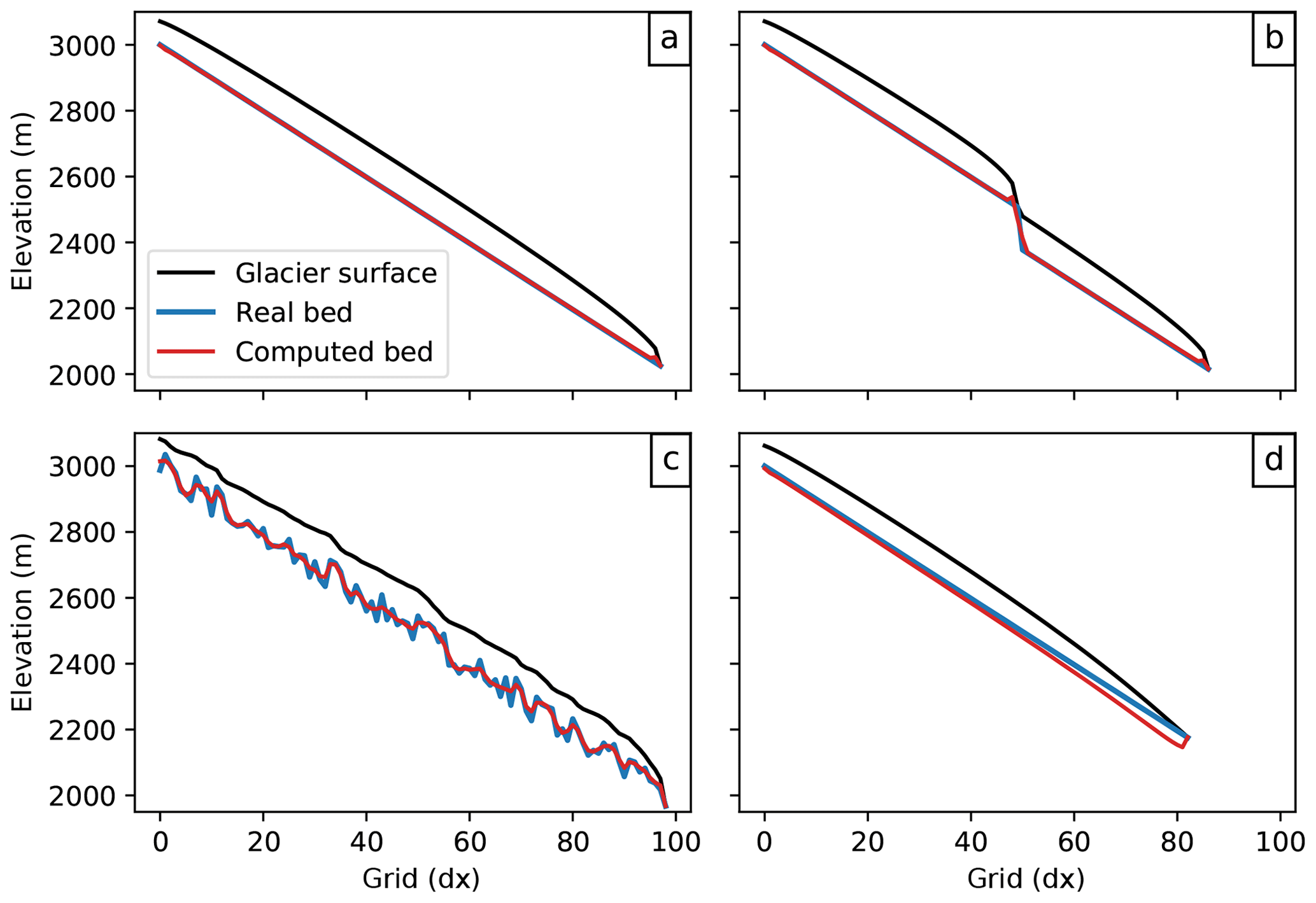
Figure 5Idealized inversion experiments: we compute the bed topography from the surface elevation obtained from a flow-line model applied to a predefined bed topography. (a–c) Glacier grown to equilibrium with different bed topographies (flat, cliff, random). (d) Transient experiment with a shrinking glacier. The same mass-balance profile is used for all experiments (linear gradient of 3 mm w.e. m−1, ELA altitude of 2600 m a.s.l.). For (d), the glacier is first grown to equilibrium then shrunk for 60 years after an ELA shift of +200 m.
Figure 5 displays some examples taken from the OGGM test suite, where the automated inversion procedure is applied on idealized glaciers generated with OGGM's flow-line model (see Sect. 3.5). In the equilibrium cases (Fig. 5a–c), the inverted topography is nearly perfect. Differences arise at strong surface gradients, mostly because of numerical differences (the inversion method uses a second-order central difference which tends to smooth the slope). The transient case (Fig. 5d) illustrates the consequences of the steady-state assumption: although the glacier is retreating, the constraint leads to a lowered ELA and, even with a perfectly known mass-balance gradient, results in an overestimated ice thickness (in this case, 25 %). This effect is visible everywhere, but is strongest at the tongue. The importance of the steady-state assumption on ice thickness estimates has been studied using numerical experiments (e.g., Adhikari and Marshall, 2012a) and is often compensated for by calibration in real-world applications.
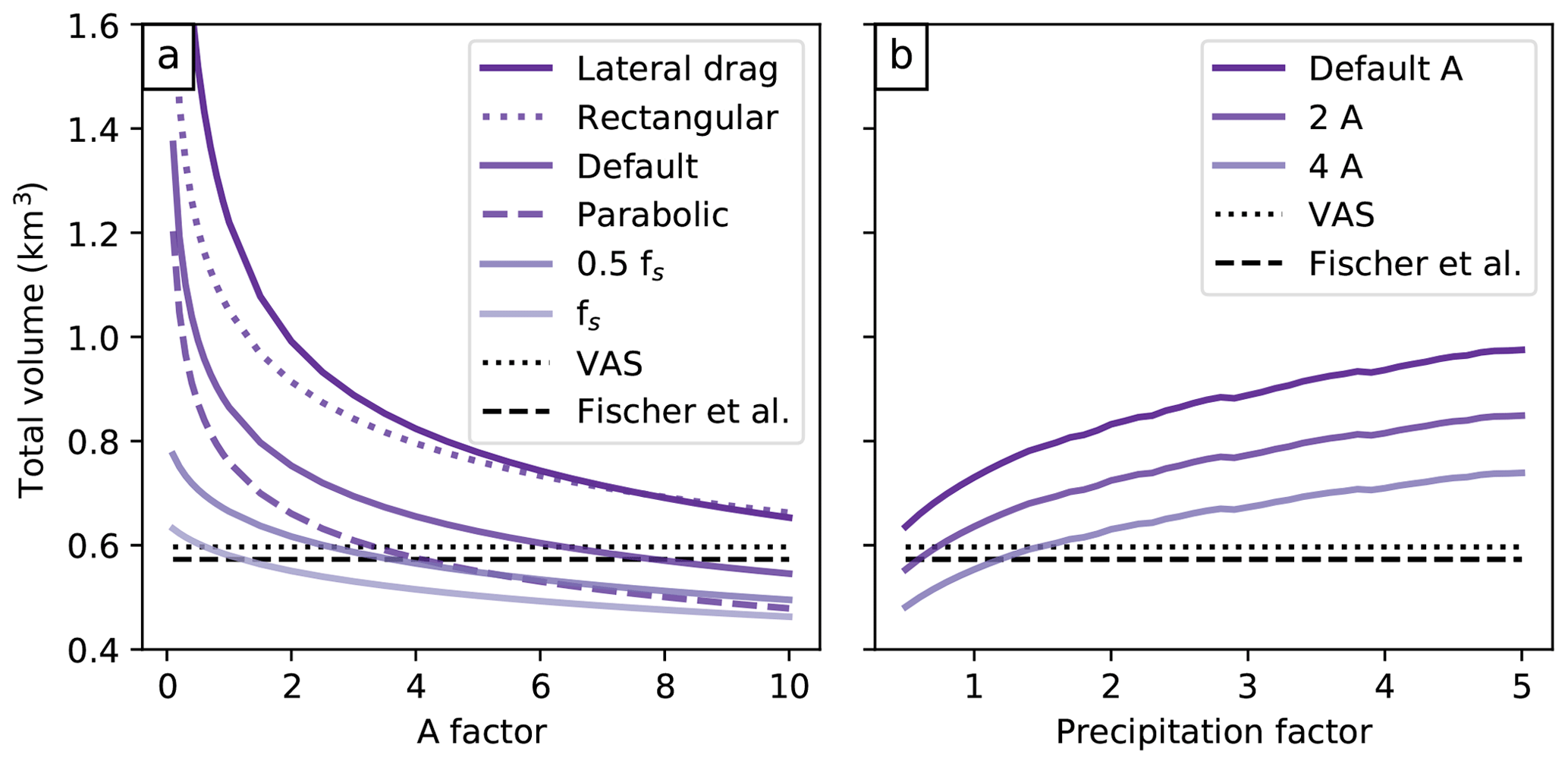
Figure 6Total volume of the Hintereisferner Glacier computed with (a) varying factors for the default creep parameter A, and (b) varying precipitation factors. The dotted and dashed black lines display the total volume estimated with volume–area scaling (VAS, Bahr et al., 1997, 2015) and based on point observations (Fischer and Kuhn, 2013). For (a), additional sensitivities are computed with an additional sliding velocity following Oerlemans (1997) using his sliding parameter fs. For (b), additional sensitivities are computed with a varying creep parameter A.
The sensitivity of the inversion procedure to various parameters is illustrated using the Hintereisferner Glacier as an example (Fig. 6). The total volume (and the local thickness) is very sensitive to the choice of the creep parameter A, varied from a factor 1∕10 to 10 times the default value of s−1 Pa−3 (Cuffey and Paterson, 2010). With a smaller A, the ice is stiffer and the glacier gets thicker (A is expected to get smaller by one or more orders of magnitude with colder ice temperatures). Inversely, softer ice leads to a thinner glacier. The shape of the curve is proportional to the fifth root of the fraction 1∕A, explaining why the volume gets very sensitive to small values of A. Adding sliding reduces the original thickness significantly for the same reasons as an increasing A, as both sliding and ice rheology (A) have a strong influence on the computed ice flux q. Inversely, adding lateral bed stresses reduces ice velocity and increases the computed ice volume. Changing from a rectangular to a parabolic bed shape yields a volume loss of approximately one-third, which is expected from geometrical considerations. The mixed parabolic/rectangular bed shape model implemented by default therefore lies in between.
The total precipitation amount, by acting on the mass-balance gradient and therefore on the ice flux q will also play a non-negligible role for the ice thickness (Fig. 6b). The effect is small in comparison to the influence of A, but it is noticeable: glaciers located in maritime climates (with high values of accumulation) will be thicker on average than similar glaciers in drier conditions.
This example shows that one can always find an optimum (and nonunique) set of parameters leading to the correct total volume. In practice, however, calibrating the model for accurate global glacier volume estimates is a major challenge for global glaciological models and will be the topic of a separate study. The IACS Working Group on Glacier Ice Thickness Estimation5 is working towards this goal: OGGM participated in the first Ice Thickness Models Intercomparison eXperiment (ITMIX, Farinotti et al., 2017), ranking amongst the best models with limited data requirements.
3.5 Ice dynamics
At this stage of the processing workflow, the ice-dynamics module is straightforward to implement. Provided with the mass balance, slope, width w, and bed topography along the flow line, we solve
numerically with a forward finite difference approximation scheme on a staggered grid. Numerical stability is ensured by the use of an adaptive time stepping scheme following the Courant–Friedrichs–Lewy (CFL) condition with γ as the dimensionless Courant number chosen between zero and one. Unlike many solvers of the shallow-ice equation, we do not transform Eq. (7) to become a diffusivity equation in h, but solve it as it is formulated here. This has the advantage that the numerical solver is the same regardless of the shape of the bed (parabolic, trapezoidal, or rectangular). The new section S at time t+Δt allows for the computation of h(t+Δt) according to the local bed geometry. Therefore, it is possible to have changing bed geometries along a single flow line using the same numerical solver. The drawback of our approach is that we cannot take advantage of the diffusivity equation solvers already available elsewhere. We tested our solution against the robust and mass-conservative solver presented by Jarosch et al. (2013). Our model yields accurate (and faster) results in most cases, but fails to ensure mass-conservation for very steep slopes like most other solvers to date. While a flow-line version of the solver presented by Jarosch et al. (2013) is available in OGGM, it is not used operationally as it cannot yet handle varying bed shapes and multiple flow lines – it will become the default solver when these elements are implemented.
At a junction between a tributary and its downstream line, an artificial grid point is added to the tributary line. This grid point has the same section area S and thickness h as the previous one, but the surface slope is computed from the difference in elevation between the tributary and descendant flow line. This is necessary to ensure a dynamical connection between the two lines: when the main flow line is at a higher elevation than its tributary, no mass exchange occurs and the tributary will build up mass until enough ice is available. At a junction point, Eq. (7) therefore contains an additional mass flux term from the tributary.
Before the actual run, a final task merges the output of all preprocessing steps and initializes the flow-line glacier for the model. For the glaciers to be allowed to grow, a downstream flow line is computed using a least cost routing algorithm leading the glacier towards the domain boundaries (this algorithm is similar to the algorithm used to compute the glacier centerlines). The bed geometries along the downstream line are computed by fitting a parabola to the actual topography profile. In the case of bad fit, the values are interpolated or a default parabola is used. Along the glacier, where the bed geometries are unknown before the inversion, the bed geometries are either rectangular (ice divides and junctions) or parabolic. Very flat parabolic shapes can occasionally occur, for wide sections with a shallow ice thickness. These geometries are unrealistically sensitive to changes in h. They create a strong positive feedback (the thickening of ice leading to a highly widening glacier) and are therefore prevented: when the parabola parameter falls below a certain threshold, the geometry is assumed to be trapezoidal instead.
The coupling between the mass balance and ice dynamics modules is a user choice. The spatially distributed mass balance used by the dynamical model can be updated (i) at each time step of the dynamical model's computation, (ii) each month, (iii) each mass-balance year (the default), or (iv) only once (for testing and feedback sensitivity investigations). In practice, this does not make much difference for the yearly averages of glacier change (except for option iv), and the choice of a yearly update is mostly driven by performance considerations. Note that the mass-balance model can compute the mass balance at shorter time intervals if required by the physical parameterizations, as the interface between the model elements simply requires the mass-balance model to integrate the mass balance over a year before giving it to the dynamical model.
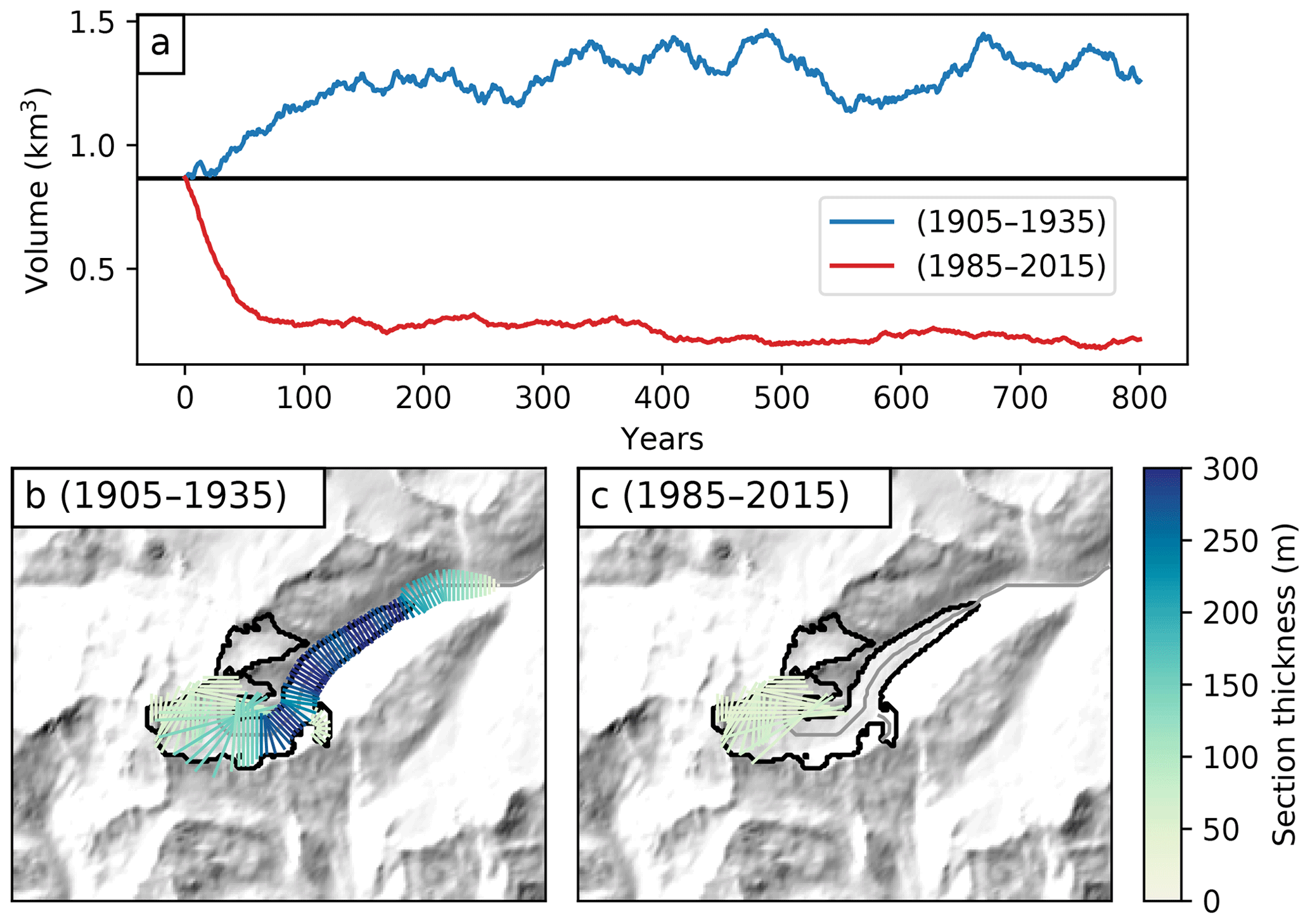
Figure 7Evolution of the Hintereisferner Glacier under two random forcing scenarios and for the default parameter set. For each scenario, the “climate years” during a 31-year period are shuffled randomly, creating a realistic climate representative for a given period. (a) The glacier volume evolution for each scenario (the black line marks the initial computed glacier volume). (b, c) The glacier shape at the end of the 800-year simulation for each case.
The results of two idealized simulations with an advancing and a shrinking scenario are shown in Fig. 7. When put under the cold and wet climate of the beginning of the 20th century, Hintereisferner Glacier would grow about two-thirds larger than it is today. Inversely, the glacier is in strong disequilibrium with today's climate, and it would lose about two-thirds of its volume if the climate remained as it was over the past 31 years. The response time of the glacier is approximately twice as fast in the shrinking case, and the natural random variations of the glacier are much smaller than for a large glacier with more inertia and a longer response time.
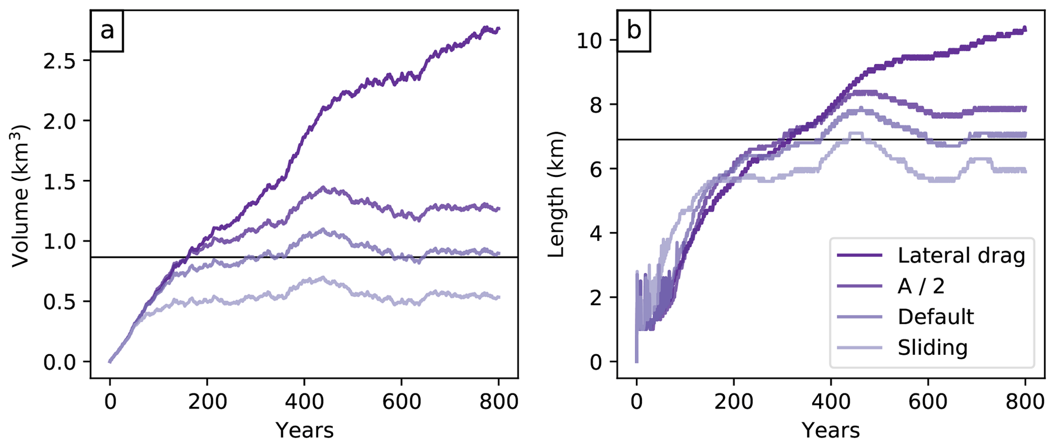
Figure 8Evolution of volume (a) and length (b) of Hintereisferner Glacier under a random climate forcing generated by shuffling the “climate years” representative for the 31-year period centered on t*. The glacier is reset to zero for each simulation, and the bed topography is obtained using the default parameters. The sensitivity to the addition of a sliding velocity or to a halving of the creep parameter A are also shown. The noisy patterns of the length time series are due to the fact that the length of a glacier on a discrete grid is sensitive to small interannual variations.
The previous results were obtained with the default setup of OGGM. In Fig. 8 we assess the sensitivity of the dynamical model to changes in the creep parameters A and to the addition of lateral drag and basal sliding velocity. As expected, these dynamical parameters affect the equilibrium volume and the response time of the glacier (faster ice leading to a thinner glacier, and visa versa). Due to the mass-balance–elevation feedback, the stiffer and therefore thicker glacier is also larger and longer, but its response to climate variability is smaller in amplitude than that of the fast moving sliding glacier.
A and fs depend on many factors such as ice temperature or basal characteristics and they cannot be assumed to be globally constant. They are considered as calibration parameters in OGGM, and will be tuned towards observations of ice thickness or glacier length changes. In this study we only calibrate the mass-balance model while the ice dynamics parameters are set to their default values ( s−1 Pa−3, fs=0, no lateral drag). Nevertheless, we discuss the model sensitivity to these dynamical parameters for individual glaciers (Fig. 8) or global runs (Fig. 10).
3.6 Special cases and model limitations
The previous experiments demonstrate that the OGGM model is capable of simulating the dynamics of glaciers in a fully automated manner. In this section we describe the implications of the flow-line approximation in the special cases of water-terminating glaciers and ice caps, and discuss some examples of glaciers with a less trivial geometry.
3.6.1 Water-terminating glaciers
Glaciers are defined as “water-terminating” in OGGM when their RGI terminus attribute is either flagged as marine-terminating or lake-terminating. The major difference between a water-terminating glacier and a valley glacier is the additional mass loss that occurs at the glacier front (frontal ablation). This has implications for the bed thickness inversion, which currently assumes that the mass flux at the front is zero (by setting , see Sect. 3.4), and for the dynamics of the glacier. The current treatment of water-terminating glaciers in OGGM is very simple but explicit. We do not take frontal ablation into account for the bed inversion (i.e., the original glacier front has a thickness of zero), but we do have a basic parameterization in the ice dynamics module. We add a grid point behind the glacier front which is reset to zero ice thickness at each time step: the ice mass suppressed this way is the frontal ablation flux, which we store. This parameterization has the advantage of preventing water-terminating glaciers from advancing while still allowing them to retreat (in which case they stop calving). We are working on a more advanced frontal ablation parameterization for both the ice dynamics and the ice thickness inversion (Recinos et al., 2018).
3.6.2 Ice caps and ice fields
Ice caps and ice fields in the RGI are divided into single dynamical entities separated by their ice divide (Fig. 9). However, the entities that belong to an ice cap are classified as such in the RGI; currently, the only special treatment for these entities in OGGM is that only one major flow line is computed (without tributaries). Indeed, the geometry of ice caps is often non-trivial, and it is not clear whether tributaries would really improve the model results. An example of an ice cap is shown in Fig. 9. While the general behavior of this ice cap is reasonably simulated by the flow-line model (e.g., at the outlet glaciers), other features appear to be unrealistic (e.g., close to the ice divides). Moreover, the mass-conservation inversion method probably underestimates the real ice thickness at the location of the ice divide, where other processes related to the past history of the ice cap are at play. A possible way forward would be to run a distributed shallow-ice model instead of the flow-line representation, and it is part of our long-terms plans to do so.
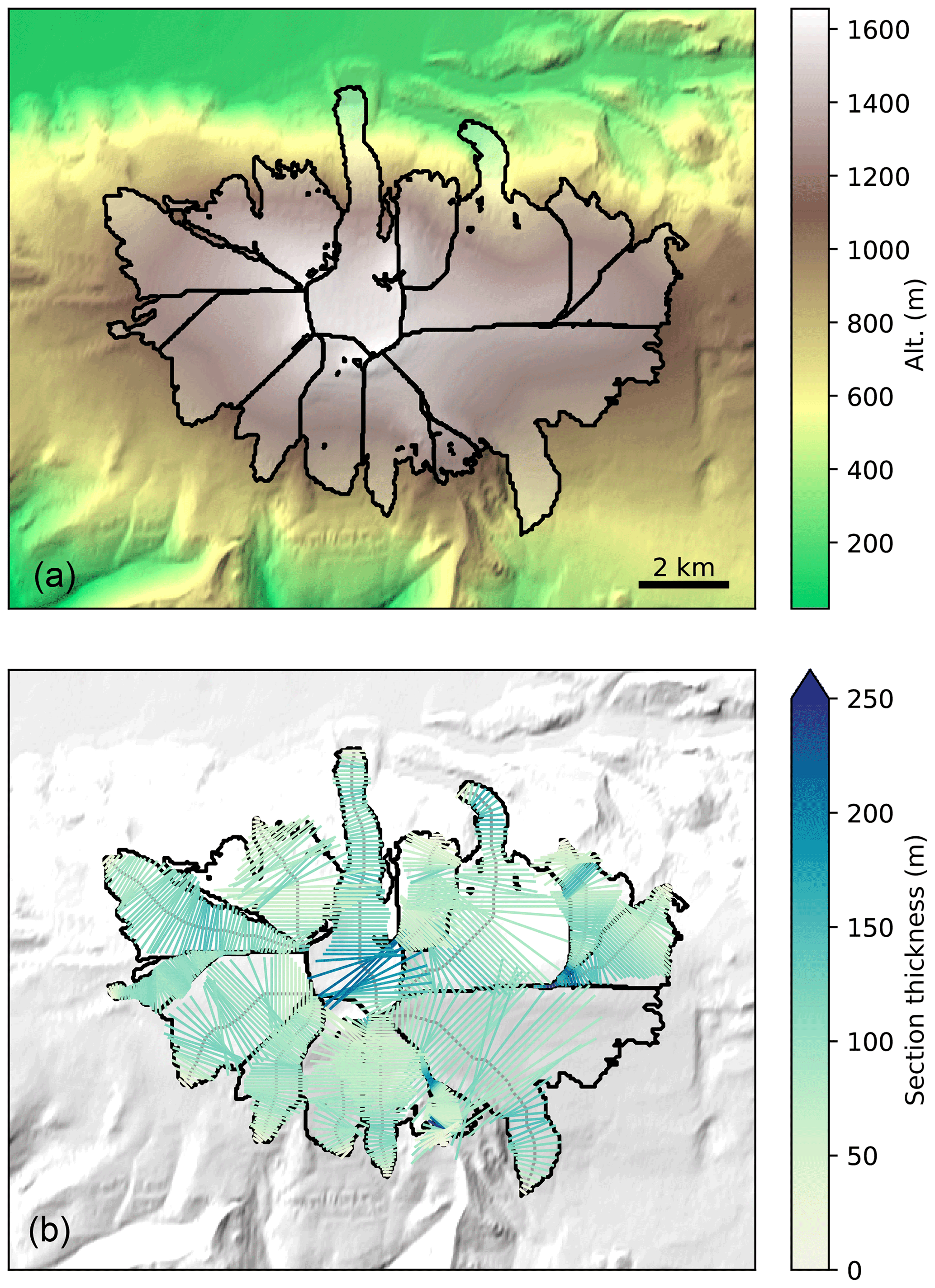
Figure 9The OGGM inversion workflow applied to the RGI entities of the Eyjafjallajökull ice cap, Iceland. (a) Outlines and topography. (b) Glacier thickness.
3.6.3 Glacier complexes
Single glaciers can be defined as the smallest dynamically independent entity, i.e., the boundaries between two glaciers should approximately follow the ice divides or hydrological basin boundaries. The flow-line assumption strongly relies on this condition being true, and indeed most of the RGI glaciers are properly outlined. Unfortunately there are notable exceptions, for three main reasons:
-
Human decision: some well known glaciers have historical boundaries that the inventory provider wanted to keep, although the glacier is now divided in smaller entities. A good example is the Hintereisferner Glacier (Fig. 7), which should have three outlines instead of one.
-
Uncertainties in the topography: the inventories are often generated using both automated processes and manual editing. There is no guarantee that we use the same DEM as the original inventory, and therefore OGGM and RGI might disagree on the ideal position of an ice divide.
-
Unavailable data: some remote glaciers and ice caps are outlined in the RGI, but not divided at all. These are the most problematic cases, and should be a matter of concern for all RGI users. For example, the largest glacier in RGI (an ice cap in northeastern Greenland with the ID RGI60-05.10315 and an area of 7537 km2) is wrongly outlined and should be separated into at least a dozen smaller entities.
Most of the small errors are filtered out by OGGM with algorithms based on surface slope thresholds (see Sect. 3.2), but the latter group of glaciers should be handled upstream. We have developed an open-source tool to automatically compute glacier divides (https://github.com/OGGM/partitioning, last access: 27 February 2019, based on Kienholz et al., 2013), but do not use it here. This issue is a large source of uncertainty for ice thickness estimates and dynamical modeling of glaciers in general, and could be the subject of a dedicated study.
3.6.4 Glacier centric modeling
Like most global glacier models, OGGM simulates each glacier individually. This has evident practical advantages, and is also a strong asset for our mass-balance model calibration algorithm. However, this has two major drawbacks: (i) neighboring glaciers will not merge although they grow together, and (ii) we can only simulate glaciers which are already inventoried, whereas uncharted glaciers are simply ignored. Both errors are a source of uncertainty for long or past simulations but less so for short-term projections in a warming world. The most obvious way to deal with this issue is to use distributed models (e.g., Clarke et al., 2015), with their own drawbacks (e.g., computational costs and the need for distributed mass-balance fields). Another way would be to allow the dynamical merging of neighbor flow-line glaciers at run time. While both are viable options for the OGGM workflow, they represent a considerable increase in complexity and are not available yet. Like other fundamental issues described in this paper (such as missing topographical data or wrongly outlined glaciers), this problem will also affect other glacier models. We hope that some of the tools we introduce here will help to solve some of these issues upstream, and that the community will soon be able to put pressure on commercial data providers for better data availability.
Thanks to its automated workflow, OGGM is able to apply all of the processes described in the previous section to all glaciers globally with the exception of Antarctica, where no CRU data are available (see Appendix C for an overview of the RGI regions). No special model setup is needed, and we use all model default settings without any calibration (this is not strictly true for the μ* calibration, which is an automated process and cannot be tuned or turned off). In the following analyses the focus is placed on the model behavior and not on the quantitative results. However, in the following we show that our results are close to expectations even without calibration, indicating realistic model behavior.
4.1 Hardware requirements and performance
Thanks to the computational efficiency of the flow-line model, OGGM runs quickly enough to be used on a personal computer for up to several dozen glaciers. At the global scale a high performance computing environment is required. For these global simulations we used a small cluster comprising two nodes with 16 quad-core processors each, resulting in 128 parallel threads. With this configuration, the model preprocessing chain (including the ice thickness inversion) takes about 7 h to complete (without data download). The total size of the (compressed) preprocessed output is 122G, which can be reduced by deleting intermediate computing steps. The amount of required storage increases with each dynamical run; here again it is possible to reduce the amount of data by only storing diagnostic variables, such as volume, area, length, and ELA, instead of the full model output. The dynamical runs are the most expensive computations: running five 300-year-long global runs takes about 24 h on our small cluster, which is a very satisfying performance. It is interesting to note that because of the adaptive time step, glacier shrinkage scenarios run faster than growing ones.
4.2 Invalid glaciers
Due to uncertainties in the input data (topography, outlines, climate), a certain number of glaciers fail to be modeled by OGGM. The statistics of these invalid glaciers are summarized in Table 1. The largest number of errors (2.6 % of the total area) are due to invalid climate series. Errors mostly occur when the climate is too cold for melt to occur or, inversely, too warm or too dry for accumulation to take place. While some of these errors are directly due to incorrect climate data, some can also be attributed to missing processes in the OGGM mass-balance model, such as sublimation and frontal ablation, which both lead to mass loss even at cold temperatures. The least problematic source of error (0.2 % of the total area) is due to failures during the actual dynamical run. The large majority of dynamical failures (751 out of 772) happen because the glacier exceeded the domain boundaries at run time. Some of these errors could be mitigated by increasing the domain size (at the cost of computational efficiency). Only 21 glaciers fail due to numerical instabilities. Finally, there are a number of other errors (0.3 % of the total area) occurring at other stages of the model chain. Examples include errors in processing the geometries or failures in computing certain topographical properties due to invalid DEMs. In total, 7084 glaciers (3.1 % of the total area) cannot be modeled by the OGGM. There are strong regional differences, with remote high and low latitude regions accounting for most of the errors.
Table 1Statistics of the model errors for each RGI region. The column names indicate which processing step produces an error, the value is the number of invalid glaciers and (in parentheses) the percentage of regional area they represent.

4.3 Volume inversion
A summary of the volume inversion results is presented in Fig. 10. As expected from theory (Bahr et al., 1997, 2015), our glacier volume estimates approximately follow a power law relationship with the glacier area (V=cSγ). The coefficients obtained by a linear fit in log space are close, but not equal to the coefficients computed by Bahr et al. (1997). In particular, the OGGM fit is slightly flatter than the theoretical value (Fig. 10a), in accordance with empirical coefficients (e.g., Bahr et al., 2015; Grinsted, 2013). This is an encouraging result, especially because it was reached using the OGGM default settings and without calibration.
The global volume estimates are particularly sensitive to the choice of the ice dynamics parameters, as shown in Fig. 10b. As for individual glaciers, the total volume follows an inverse polynomial curve as expected from the equations of ice flow. Changing from a rectangular to a parabolic bed shape yields a volume loss of exactly one-third (see Sect. 3.4). Adding lateral drag yields a volume very close to the rectangular case, and, although this is fortuitous (individual glaciers can show different results, see Fig. 6), it matches the original purpose of the parameterization nicely, which is to compute a more realistic ice flow for parabolic bed shapes. The three independent estimates plotted as straight dotted lines (VAS; Huss and Farinotti, 2012; Grinsted, 2013) illustrate that A is a relatively straightforward parameter to act upon in order to fit the model to observations. The effect of A, however, is going to be the same on all glaciers and therefore will be a poor measure of performance (see also Bahr et al., 2015, Sect. 8.11). In fact, the added value of OGGM is more likely to be found in the deviations from the scaling law (Fig. 10b). The deviations are the result of a range of possible factors such as slope, total accumulation, or altitude area distribution. With accurate boundary conditions, OGGM should be able to provide more accurate estimates, within the limits of the assumptions and simplifications behind the model equations. The calibration and validation of the OGGM inversion model will be the topic of a subsequent study.
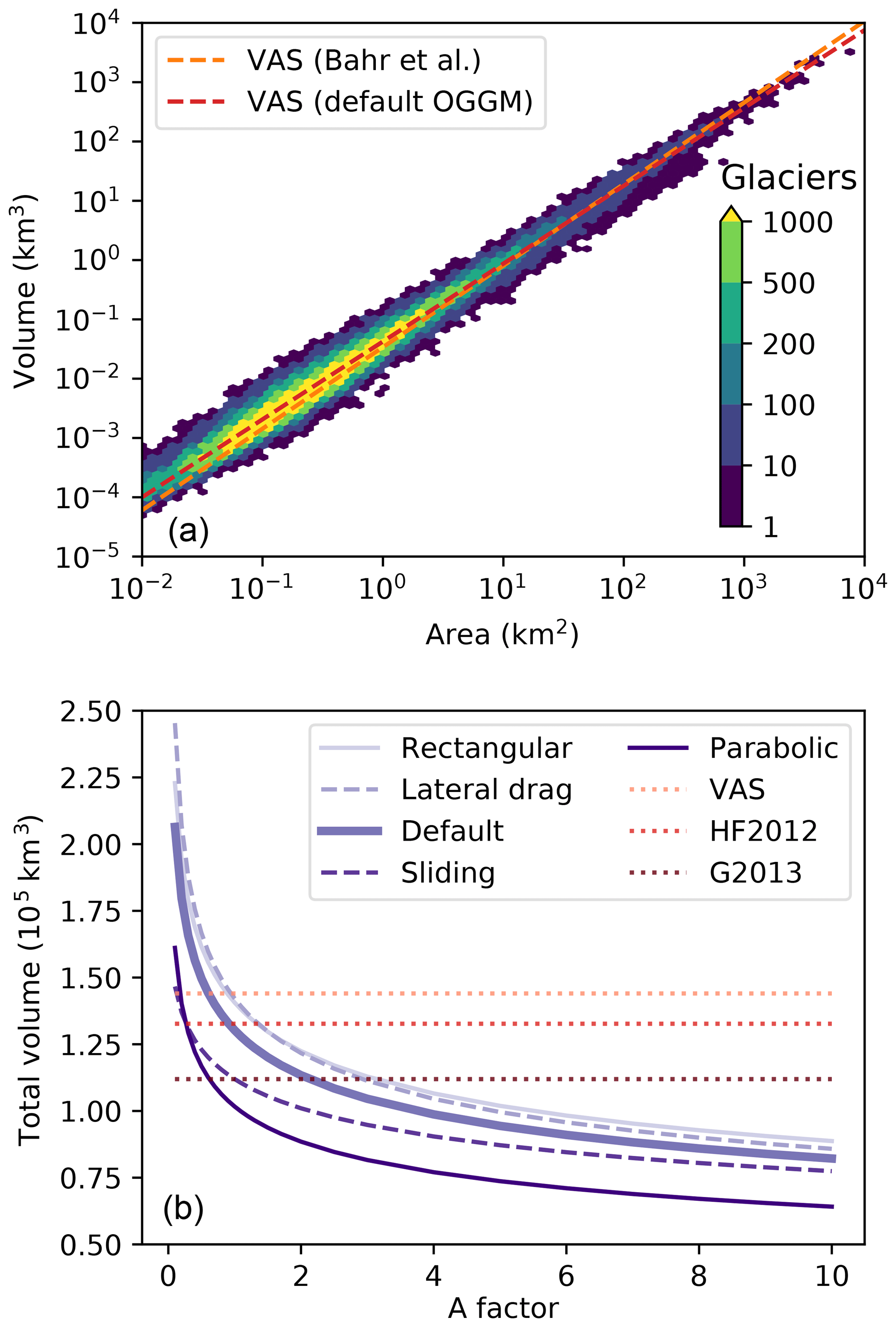
Figure 10Global glacier volume modeling. (a) Binned scatterplot of volume versus area for all valid glaciers (N= 207 438) using the default OGGM setup. Color shading indicates the number of glaciers in each bin. Note the logarithmic scale of the axes and the irregular color scale levels. The dashed lines indicate the volume–area scaling relationship with either the theoretical parameters from Bahr et al. (1997) (V=0.034 S1.375) or fitted on our own data (V=0.042 S1.313). (b) Global volume estimates as a function of the multiplication factor applied to the ice creep parameter A, with five different setups: defaults, with sliding velocity, with lateral drag, and with rectangular and parabolic bed shapes only (instead of the default mixed parabolic/rectangular). In addition, we plotted the estimates from standard volume–area scaling (VAS, V=0.034 S1.375), Huss and Farinotti (2012) (HF2012) and Grinsted (2013) (G2013). The latter two estimates are provided for indication only as they are based on a different glacier inventory.
4.4 Dynamical runs
We test the model behavior by running several 300-year-long global simulations under various climate “scenarios”. In the first simulations (Fig. 11), we run the model under the climate of the past 31 years. In order to keep the forcing realistic, we create a pseudo-random climate by shuffling the years infinitely. We also run two additional simulations with a 0.5 ∘C positive and negative bias. The unbiased simulation illustrates the committed glacier mass loss, i.e., the ice mass which is not sustainable under the current climate. Figure 11 shows that all regions will continue to lose ice even if the climate remains constant. The regions with the largest committed mass loss relative to the initial volume are western Canada and US (02), Svalbard (07), and the three “High Mountain Asia” regions (13, 14, and 15). Conversely, the Arctic Canada south (04), Greenland (05), and Iceland (06) regions are least affected. The reasons for these regional differences are complex; they are due to the climate itself of course, but also to glacier properties such as size, slope, and continentality. The regions that are far from equilibrium also tend to be less sensitive to the temperature bias experiments, although this should not be overinterpreted (indeed, the range of the y axes can hide differences which appear small in comparison to the large regional glacier loss).
In general, the model behavior looks reasonable and the regional differences are in qualitative agreement with other global studies (e.g., Huss and Hock, 2015, where the regions with a stronger response to 21st century climate change are the same as those listed above). Furthermore, our global estimate of the committed mass loss (approx. 33 % at the end of the 300-year simulation, probably more at equilibrium) is in agreement with other studies (27±5 %, 38±16 %, and 36±8 % for Bahr et al., 2009; Mernild et al., 2013; Marzeion et al., 2018, respectively).
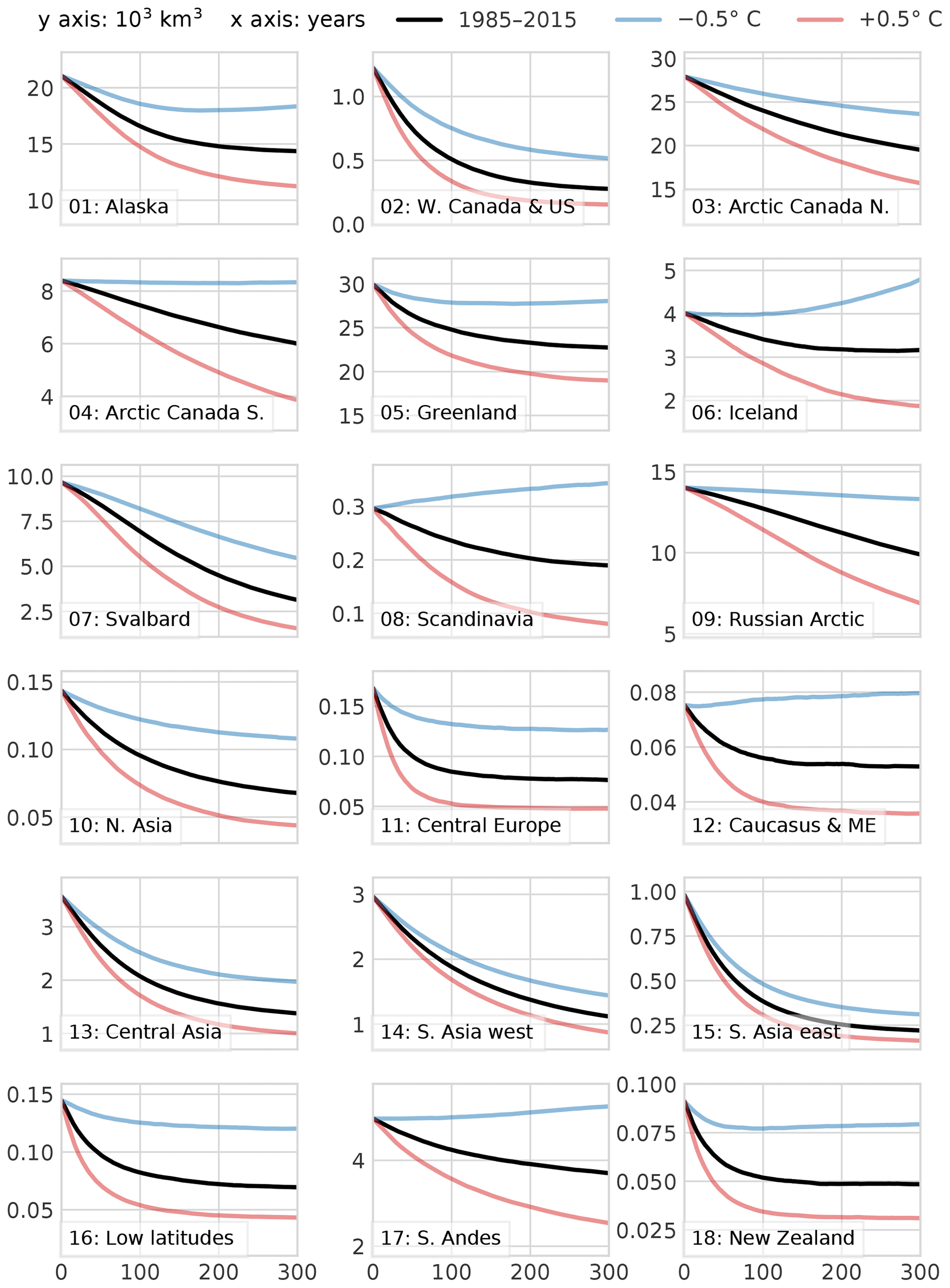
Figure 11Regional glacier volume change under the 1985–2015 climate (randomized) with three temperature biases (−0.5∘, 0∘, and +0.5∘). Note the units of the y axes (103 km3) and the marked regional differences.
A further model test is presented in Fig. 12. Here, we apply a new climate scenario: the climate at t* which, for each glacier individually, represents a theoretical equilibrium climate. In addition to the global response to these scenarios, we separate between the majority group of smaller glaciers and the much smaller group of very large glaciers. Both groups are selected so that they sum up to one-quarter of the total glacier volume. A striking feature of the runs is that the glaciers tend to grow under the artificial t* climate. The growth is slow at first and accelerates with time, hinting towards a positive feedback. This feedback is driven by two factors: first, a higher surface elevation leads to a positive change in mass balance (mass-balance–elevation feedback); and second, due to the parabolic and trapezoidal bed shapes, a larger ice thickness leads to a wider accumulation area above the ELA and to a wider ablation area below the ELA. It appears that the positive width–accumulation feedback is stronger than the negative width–ablation feedback. This can be explained by the larger accumulation area of glaciers in an equilibrium climate: the average accumulation area ratio at t* in OGGM is 51 %. In order to test which of these feedbacks is stronger, we run a simulation with rectangular bed shapes exclusively (dotted light purple line in Fig. 12), thereby eliminating the width–accumulation but keeping the mass-balance–elevation feedback. The results show that for the vast majority of glaciers the feedback almost disappears, whereas the very large glaciers still show a weak and delayed altitude feedback.
It is unclear whether this is a bug or a feature. On the one hand, this behavior is not really desirable as one would expect glaciers to remain constant under a theoretical equilibrium climate. On the other hand, t* is just a vehicle to calibrate the model and was not supposed to yield a particular insight (for example, many glaciers can only have an equilibrium t* climate after the application of a bias to the operational mass-balance model). There are many reasons why small initial perturbations such as numerical noise or the differences between the bed inversion and forward model numerical schemes might lead to a different equilibrium. It must also be noted that this feedback is slow to appear, and will only have a notable influence on the largest glaciers for long-term simulations in a cooler climate (the global volume change after 100 years due to the feedback is 2.4 % for the default and 1 % for the all rectangular cases). The very simple definition of an “equilibrium climate” for these very large glaciers is problematic anyway: large glaciers have a very slow but potentially large response to the smallest changes in climate. At the global scale, most of the 300-year volume loss is due to the small glaciers, which respond faster and stronger than larger ones.
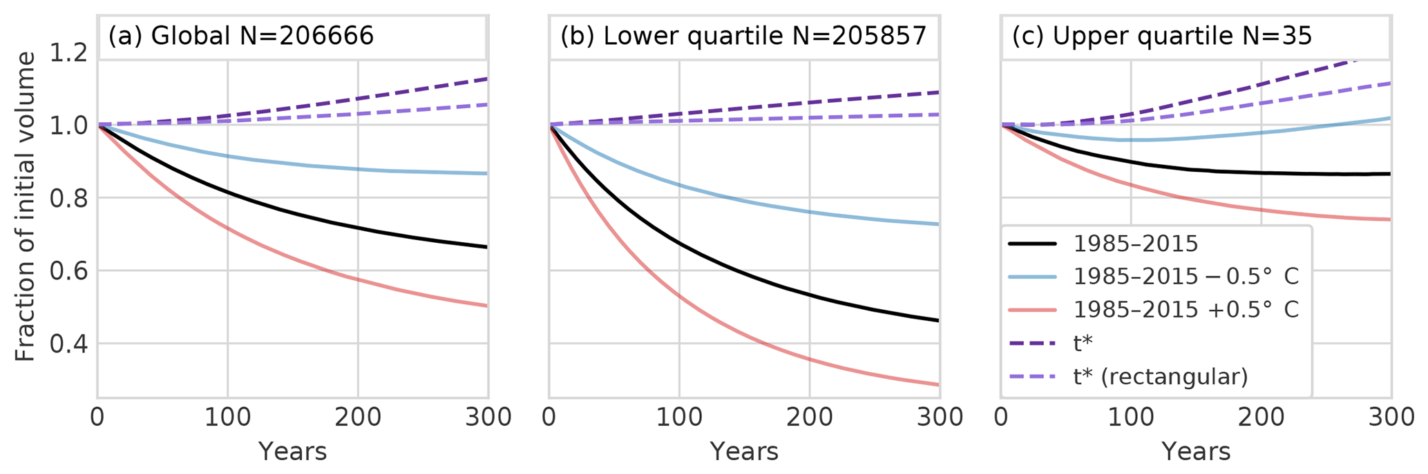
Figure 12(a) Global glacier volume change under various climate scenarios (1985–2015 climate with three temperature biases and climate at t* which, for each glacier individually, represents a theoretical equilibrium climate) and model configurations (rectangular bed instead of the mixed default), plotted as a fraction of the initial volume. (b, c) Volume changes of all glaciers making up for the first and last quartile of the sorted cumulative total volume.
We present a new model of global glacier evolution, the Open Global Glacier Model (OGGM, v1.1). The panoply of tools available to compute past and future glacier change range from simple box models (e.g., Harrison, 2013) to more complex, geometry aware models (Huss and Hock, 2015, to cite the most recent in date). OGGM undoubtedly belongs to the complex side of this scale. Different model complexities are justified by different problem settings, taking the model-specific merits and drawbacks into account. Instead of endorsing one approach over the other, OGGM aims to provide a framework which allows one to switch between models and allows objective intercomparisons. In fact, the ice dynamics module represents only a small fraction of the OGGM code base: a huge amount of work has been invested to provide a series of tools which will help others in their own modeling endeavors. Any interested person can download, install, and run these tools at no cost. This includes the automated download of topographic and climate data for any location on the globe, the collation of glacier attributes, the automated computation of glacier centerlines, or the delineation of glacier dynamical entities. While some of these tools have been described elsewhere, the added value of OGGM is that they are now centralized, documented, and available for public review via the open-source model.
In the future, we will continue to encourage external contributions in several ways. First, it must be as easy as possible for a new user to detect where and how a contribution can be implemented; hence, documentation is key. Then, the model must be able to cope with different ways of simulating a considered process: every single task in the OGGM workflow can be replaced or enhanced, as long as the format of the input and output files is agreed upon beforehand. Perfect modularity will be hard to achieve, but the recent implementation of alternative numerical solvers show that modularity is possible. Finally, we need to ensure attribution to the original contribution (e.g., a scientific publication) in order to engage the wider community. For this purpose, we developed a template repository for external OGGM modules: https://github.com/OGGM/oggmcontrib (last access: 27 February 2019). This development model will ensure that users importing OGGM extensions will be aware of the source of each module they are using and will be able to refer to the original contribution appropriately. We hope that this development model will foster new collaborations.
We cannot (and do not want to) demonstrate that OGGM will provide more accurate estimates of future sea-level rise than earlier attempts. However, OGGM allows new studies which were not previously possible. The dynamical representation of glacier advance and retreat enables studies of glacier evolution at long (paleo-) timescales, where ice dynamics and geometrical attributes such as the accumulation area ratio play an important role (e.g., Mackintosh et al., 2017). The first OGGM simulations over the last millennium show very promising results (Goosse et al., 2018). The modular framework allows one to compare the performance of various parameterizations such as the mass balance and downscaling algorithms. It may be argued that the amount of available data is not sufficient to constrain modeling studies such as ours at the global scale. The OGGM can now be used to test this argument by allowing simpler modules to be added to the code base and test the added value of increased complexity.
Planned and envisioned future developments for the model follow the general guidelines of modularity and extendability. While some of the authors are working on adding even more complexity to the model (for example by improving the frontal ablation and mass-balance parameterizations or by implementing a distributed ice dynamics module), it is part of our plans to implement simpler approaches, such as the original Marzeion et al. (2012b) model or the Huss and Farinotti (2012) approach to ice thickness estimation. A considerable amount of work will be needed to correctly assess the uncertainties associated with the model chain; therefore, Monte Carlo and Bayesian approaches might be the best courses of action.
The non-linear dynamical behavior of glaciers raises a wide range of very interesting inverse problems. For example, how to deal with the transient climate issue in the ice thickness inversion algorithm? How much information about past climate can be extracted from moraine proxies and today's glacier extent? What are the uncertainties associated with global sea-level rise estimates, and where do they originate? How much complexity is appropriate? These are all questions that the authors hope will be easier to address through the publication of the OGGM.
The OGGM software is coded in the Python language and licensed under the GPLv3 free software license. The latest version of the code is available on GitHub (https://github.com/OGGM/oggm, last access: 27 February 2019), the documentation is hosted on Read the Docs (http://docs.oggm.org, last access: 27 February 2019), and the project website for communication and dissemination can be found at http://oggm.org (last access: 27 February 2019). The OGGM version used for this study is version 1.1 (Maussion et al., 2019). Past and future OGGM versions will be available from a permanent DOI repository (https://zenodo.org/badge/latestdoi/43965645, last access: 27 February 2019). The software ships with an extensive test suite which can be used by the users to test their configuration. The tests are triggered automatically at each new code addition, reducing the risk of introducing new bugs (https://travis-ci.org/OGGM/oggm, last access: 27 February 2019). The suite contains unit tests (for example for the numerical core) and integration tests based on sets of real glaciers. At the time of writing, 85 % of all relevant lines of code are covered by the tests (i.e., called at least once by the test suite). The remaining 15 % are challenging to monitor because they mostly concern the automated downloading tools which are used in production and cannot be tested automatically.
The following open-source libraries have to be installed in order to run
OGGM: numpy/scipy (van der Walt et al., 2011),
scikit-image (van der Walt et al., 2014), shapely
(Gillies, 2007), rasterio (Gillies, 2013), pandas
(McKinney, 2010), geopandas, xarray (Hoyer and Hamman, 2017),
pyproj, matplotlib (Hunter, 2007), and salem
(Maussion et al., 2017). OGGM runs on all major platforms (Windows, Mac, and
Linux) but we recommend using Linux as this is the platform it is most tested
on. The code and data used to generate all figures and analyses in this paper
can be found at Maussion (2019).
The default climate dataset used by OGGM is the Climatic Research Unit (CRU) TS v4.01 dataset (Harris et al., 2014, released 20 September 2017). It is a gridded dataset at 0.5∘ resolution covering the period from 1901 to 2016. The dataset is obtained by interpolating station measurements; therefore, it does not cover the oceans and Antarctica. The TS dataset is further downscaled to the resolution of 10′ by applying the 1961–1990 anomalies to the CRU CL v2.0 gridded climatology (New et al., 2002). This step is necessary because the TS datasets do not contain altitude information, which is needed to compute the temperature at a given height on the glacier. To compute the annual mass balances we use the hydrological year convention (the year 2001 being October 2000 to September 2001 in the Northern Hemisphere and April 2000 to March 2001 in the Southern Hemisphere).
For each glacier, the monthly temperature and precipitation time series are extracted from the nearest CRU CL v2.0 grid point and then converted to the local temperature according to a temperature gradient (default: 6.5 K km−1). No vertical gradient is applied to precipitation, but we apply a correction factor pf=2.5 to the original CRU time series (similar to Marzeion et al., 2012b). This correction factor can be seen as a global correction for orographic precipitation, avalanches, and wind-blown snow. It must be noted that this factor has little (if any) impact on the mass-balance model performance in terms of bias. This is due to the automated calibration algorithm, which will adapt to a new factor by acting on the temperature sensitivity μ*. To verify that the chosen precipitation factor is realistic, we use another metric – the standard deviation of the mass-balance time series. Comparisons between model and observations show that the model underestimates variability by about 10 %. We could tune the precipitation factor towards higher values to reduce this discrepancy but refrain to do so, as we do not want to add an additional free parameter in the model.
To calibrate and validate the mass-balance model, OGGM relies on mass-balance observations provided by the World Glacier Monitoring Service (WGMS, 2017). The Fluctuations of Glaciers (FoG) database contains annual mass-balance values for several hundreds of glaciers worldwide. We exclude water-terminating glaciers and the time series with less than 5 years of data. Not all of the remaining glaciers can be used by OGGM; we also need a corresponding RGI outline. Indeed, the WGMS and RGI databases have distinct glacier identifiers and it is not guaranteed that the glacier outline provided by the RGI fits the outline used by the local data providers to compute the specific mass balance. Since 2017, the WGMS has provided a lookup table linking the two databases. We updated this list for version 6 of the RGI, leaving us with 254 mass-balance time series.
These data are not equally distributed over the glaciated regions (see e.g., Zemp et al., 2015, and Fig. C1), and their quality is highly variable. In the absence of a better data basis (at least for the 20th century), we have to rely on them for the calibration and validation of our model. Fortunately, these data play a relatively minor role in the model calibration as explained in Sect. 3.3. For future studies it might be advisable to use independent, regional geodetic mass-balance estimates for validation as well.
A map of the RGI regions and some basic statistics are presented in Fig. C1.
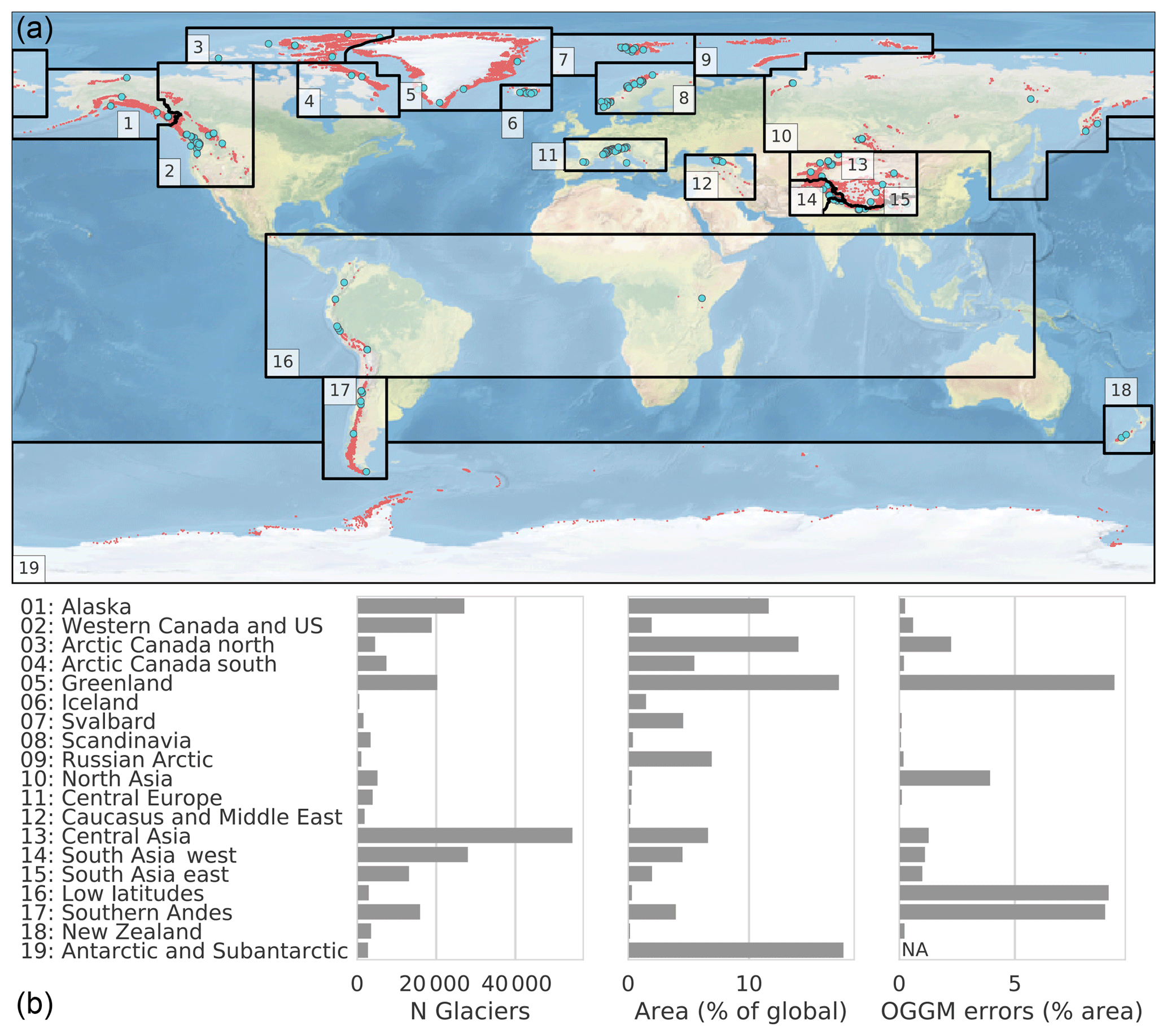
Figure C1(a) Map of the RGI regions: the red dots indicate the glacier locations and the blue circles the location of the 254 reference WGMS glaciers used by the OGGM calibration. (b) Region names and basic statistics of the database (number of glaciers per region, regional contribution to the global area in percent, and the percentage of the regional area which cannot be modeled by OGGM).
BM and FM are the initiators of the OGGM project. FM is the main OGGM developer and wrote most of the paper. AB developed the downstream bed shape estimation algorithm. NC wrote parts of the documentation. MD wrote the cross-validation monitoring website. JE developed the glacier partitioning tool. KF wrote parts of the bed inversion and dynamical cores. PG wrote the lateral drag parameterization. AJ provided a robust implementation of the dynamical core used for testing and contributed to the development of the operational scheme. JL provided the WGMS to RGI lookup table and contributed to the topographical data download tool. FO contributed to the AWS deployment tool. BR developed the frontal ablation parameterization tool. TR developed the download and parallelisation tools and is largely responsible for the successful deployment of the OGGM on supercomputing environments. AV contributed to the climate and mass-balance tools. CW provided the first implementation of the centerline determination algorithm. All authors continuously discussed the model development and the results together.
The authors declare that they have no conflict of interest.
Ben Marzeion, Johannes Landmann, and Christian T. Wild were supported by the
Austrian Science Fund (FWF), grant no. P25362. Ben Marzeion, Anton Butenko, and
Julia Eis were supported by the German Research Foundation, grant no. MA6966/1-1.
Anouk Vlug and Beatriz Recinos were supported by the DFG through
the International Research Training Group IRTG 1904 ArcTrain.
Kévin Fourteau was supported by the ENS Paris-Saclay. Nicolas Champollion
was funded by the German Federal Ministry of Education and Research (grant
no 01LS1602A). The computations were partially realized on resources provided by
Amazon Web Services Cloud Computing (sponsored by Amazon) and on the
computing facilities of the Institute of Geography, University of
Bremen.
Edited by: Didier Roche
Reviewed by: David Rounce and one anonymous referee
Adhikari, S. and Marshall, S. J.: Glacier volume-area relation for high-order mechanics and transient glacier states, Geophys. Res. Lett., 39, 1–6, https://doi.org/10.1029/2012GL052712, 2012a. a
Adhikari, S. and Marshall, S. J.: Parameterization of lateral drag in flowline models of glacier dynamics, J. Glaciol., 58, 1119–1132, https://doi.org/10.3189/2012JoG12J018, 2012b. a
Bahr, D. B., Meier, M. F., and Peckham, S. D.: The physical basis of glacier volume-area scaling, J. Geophys. Res.-Sol. Ea., 102, 20355–20362, https://doi.org/10.1029/97JB01696, 1997. a, b, c, d
Bahr, D. B., Dyurgerov, M., and Meier, M. F.: Sea-level rise from glaciers and ice caps: A lower bound, Geophys. Res. Lett., 36, 2–5, https://doi.org/10.1029/2008GL036309, 2009. a
Bahr, D. B., Pfeffer, W. T., and Kaser, G.: Glacier volume estimation as an ill-posed inversion, J. Glaciol., 60, 922–934, https://doi.org/10.3189/2014JoG14J062, 2014. a
Bahr, D. B., Pfeffer, W. T., and Kaser, G.: A review of volume-area scaling of glaciers, Rev. Geophys., 53, 95–140, https://doi.org/10.1002/2014RG000470, 2015. a, b, c, d
Budd, W. F., Keage, P. L., and Blundy, N. A.: Empirical studies of ice sliding, J. Glaciol., 23, 157–170, https://doi.org/10.1017/S0022143000029804, 1979. a
Church, J., Clark, P., Cazenave, A., Gregory, J., Jevrejeva, S., Levermann, A., Merrifield, M., Milne, G., Nerem, R., Nunn, P., Payne, A., Pfeffer, W., Stammer, D., and Unnikrishnan, A.: Sea Level Change, in: Climate Change 2013 – The Physical Science Basis, chap. 13, Intergovernmental Panel on Climate Change, Cambridge University Press, Cambridge, 1137–1216, https://doi.org/10.1017/CBO9781107415324.026, 2013. a
Clarke, G. K. C., Jarosch, A. H., Anslow, F. S., Radić, V., and Menounos, B.: Projected deglaciation of western Canada in the twenty-first century, Nat. Geosci., 8, 372–377, https://doi.org/10.1038/ngeo2407, 2015. a
Cogley, J. G.: Geodetic and direct mass-balance measurements: comparison and joint analysis, Ann. Glaciol., 50, 96–100, https://doi.org/10.3189/172756409787769744, 2009. a
Cuffey, K. and Paterson, W.: The Physics of Glaciers, 4th edn., Academic Press, 2010. a, b
Farinotti, D., Huss, M., Bauder, A., Funk, M., and Truffer, M.: A method to estimate the ice volume and ice-thickness distribution of alpine glaciers, J. Glaciol., 55, 422–430, https://doi.org/10.3189/002214309788816759, 2009. a, b, c
Farinotti, D., Brinkerhoff, D. J., Clarke, G. K. C., Fürst, J. J., Frey, H., Gantayat, P., Gillet-Chaulet, F., Girard, C., Huss, M., Leclercq, P. W., Linsbauer, A., Machguth, H., Martin, C., Maussion, F., Morlighem, M., Mosbeux, C., Pandit, A., Portmann, A., Rabatel, A., Ramsankaran, R., Reerink, T. J., Sanchez, O., Stentoft, P. A., Singh Kumari, S., van Pelt, W. J. J., Anderson, B., Benham, T., Binder, D., Dowdeswell, J. A., Fischer, A., Helfricht, K., Kutuzov, S., Lavrentiev, I., McNabb, R., Gudmundsson, G. H., Li, H., and Andreassen, L. M.: How accurate are estimates of glacier ice thickness? Results from ITMIX, the Ice Thickness Models Intercomparison eXperiment, The Cryosphere, 11, 949–970, https://doi.org/10.5194/tc-11-949-2017, 2017. a, b
Farr, T. G., Rosen, P. A., Caro, E., Crippen, R., Duren, R., Hensley, S., Kobrick, M., Paller, M., Rodriguez, E., Roth, L., Seal, D., Shaffer, S., Shimada, J., Umland, J., Werner, M., Oskin, M., Burbank, D., and Alsdorf, D.: The Shuttle Radar Topography Mission, Rev. Geophys., 45, RG2004, https://doi.org/10.1029/2005RG000183, 2007. a
Fischer, A. and Kuhn, M.: Ground-penetrating radar measurements of 64 Austrian glaciers between 1995 and 2010, Ann. Glaciol., 54, 179–188, https://doi.org/10.3189/2013AoG64A108, 2013. a
Gardner, A. S., Moholdt, G., Cogley, J. G., Wouters, B., Arendt, A. A., Wahr, J., Berthier, E., Hock, R., Pfeffer, W. T., Kaser, G., Ligtenberg, S. R. M., Bolch, T., Sharp, M. J., Hagen, J. O., van den Broeke, M. R., and Paul, F.: A Reconciled Estimate of Glacier Contributions to Sea Level Rise: 2003 to 2009, Science, 340, 852–857, https://doi.org/10.1126/science.1234532, 2013. a, b
Giesen, R. H. and Oerlemans, J.: Calibration of a surface mass balance model for global-scale applications, The Cryosphere, 6, 1463–1481, https://doi.org/10.5194/tc-6-1463-2012, 2012. a, b
Giesen, R. H. and Oerlemans, J.: Climate-model induced differences in the 21st century global and regional glacier contributions to sea-level rise, Clim. Dynam., 41, 3283–3300, https://doi.org/10.1007/s00382-013-1743-7, 2013. a, b
Gillies, S.: Shapely: manipulation and analysis of geometric objects, available at: https://github.com/Toblerity/Shapely (last access: 11 February 2019), 2007. a
Gillies, S.: Rasterio: geospatial raster I/O for Python programmers, available at: https://github.com/mapbox/rasterio (last access: 11 February 2019), 2013. a
Goosse, H., Barriat, P.-Y., Dalaiden, Q., Klein, F., Marzeion, B., Maussion, F., Pelucchi, P., and Vlug, A.: Testing the consistency between changes in simulated climate and Alpine glacier length over the past millennium, Clim. Past, 14, 1119–1133, https://doi.org/10.5194/cp-14-1119-2018, 2018. a
Gregory, J. M., White, N. J., Church, J. A., Bierkens, M. F. P., Box, J. E., Van Den Broeke, M. R., Cogley, J. G., Fettweis, X., Hanna, E., Huybrechts, P., Konikow, L. F., Leclercq, P. W., Marzeion, B., Oerlemans, J., Tamisiea, M. E., Wada, Y., Wake, L. M., and Van De Wal, R. S. W.: Twentieth-century global-mean sea level rise: Is the whole greater than the sum of the parts?, J. Climate, 26, 4476–4499, https://doi.org/10.1175/JCLI-D-12-00319.1, 2013. a
Grinsted, A.: An estimate of global glacier volume, The Cryosphere, 7, 141–151, https://doi.org/10.5194/tc-7-141-2013, 2013. a, b, c
Harris, I., Jones, P., Osborn, T., and Lister, D.: Updated high-resolution grids of monthly climatic observations - the CRU TS3.10 Dataset, Int. J. Climatol., 34, 623–642, https://doi.org/10.1002/joc.3711, 2014. a, b
Harrison, W. D.: How do glaciers respond to climate? Perspectives from the simplest models, J. Glaciol., 59, 949–960, https://doi.org/10.3189/2013JoG13J048, 2013. a
Howat, I. M., Negrete, A., and Smith, B. E.: The Greenland Ice Mapping Project (GIMP) land classification and surface elevation data sets, The Cryosphere, 8, 1509–1518, https://doi.org/10.5194/tc-8-1509-2014, 2014. a
Hoyer, S. and Hamman, J. J.: xarray: N-D labeled Arrays and Datasets in Python, J. Open Res. Softw., 5, 1–6, https://doi.org/10.5334/jors.148, 2017. a
Hunter, J. D.: Matplotlib: A 2D Graphics Environment, Comput. Sci. Eng., 9, 90–95, https://doi.org/10.1109/MCSE.2007.55, 2007. a
Huss, M.: Present and future contribution of glacier storage change to runoff from macroscale drainage basins in Europe, Water Resour. Res., 47, W07511, https://doi.org/10.1029/2010WR010299, 2011. a
Huss, M. and Farinotti, D.: Distributed ice thickness and volume of all glaciers around the globe, J. Geophys. Res.-Earth, 117, F04010, https://doi.org/10.1029/2012JF002523, 2012. a, b, c, d, e, f
Huss, M. and Hock, R.: A new model for global glacier change and sea-level rise, Front. Earth Sci., 3, 1–22, https://doi.org/10.3389/feart.2015.00054, 2015. a, b, c, d
Hutter, K.: The effect of longitudinal strain on the shear stress of an ice sheet: in defence of using streched coordinates, J. Glaciol., 27, 39–56, 1981. a
Hutter, K.: Theoretical glaciology: material science of ice and the mechanics of glaciers and ice sheets, in: Mathematical Approaches to Geophysics, Springer Netherlands, 510 pp., 1983. a
Immerzeel, W. W., van Beek, L. P. H., Konz, M., Shrestha, A. B., and Bierkens, M. F. P.: Hydrological response to climate change in a glacierized catchment in the Himalayas, Clim. Change, 110, 721–736, https://doi.org/10.1007/s10584-011-0143-4, 2012. a
Jarosch, A. H., Schoof, C. G., and Anslow, F. S.: Restoring mass conservation to shallow ice flow models over complex terrain, The Cryosphere, 7, 229–240, https://doi.org/10.5194/tc-7-229-2013, 2013. a, b
Jarvis, A., Reuter, H., Nelson, A., and Guevara, E.: Hole-filled SRTM for the globe Version 4, CGIAR Consortium for Spatial Information, University of Twente, 2008. a
Kaser, G., Grosshauser, M., and Marzeion, B.: Contribution potential of glaciers to water availability in different climate regimes, P. Natl. Acad. Sci. USA, 107, 20223–20227, https://doi.org/10.1073/pnas.1008162107, 2010. a
Kienholz, C., Hock, R., and Arendt, A. A.: A new semi-automatic approach for dividing glacier complexes into individual glaciers, J. Glaciol., 59, 925–937, https://doi.org/10.3189/2013JoG12J138, 2013. a
Kienholz, C., Rich, J. L., Arendt, A. A., and Hock, R.: A new method for deriving glacier centerlines applied to glaciers in Alaska and northwest Canada, The Cryosphere, 8, 503–519, https://doi.org/10.5194/tc-8-503-2014, 2014. a, b, c
Leclercq, P. W., Oerlemans, J., and Cogley, J. G.: Estimating the Glacier Contribution to Sea-Level Rise for the Period 1800-2005, Surv. Geophys., 32, 519–535, https://doi.org/10.1007/s10712-011-9121-7, 2011. a
Liu, H., Jezek, K. C., Li, B., and Zhao, Z.: Radarsat Antarctic Mapping Project Digital Elevation Model, Version 2, Boulder, Colorado USA, NASA National Snow and Ice Data Center Distributed Active Archive Center, https://doi.org/10.5067/8JKNEW6BFRVD, 2015. a
Mackintosh, A. N., Anderson, B. M., and Pierrehumbert, R. T.: Reconstructing Climate from Glaciers, Ann. Rev. Earth Planet. Sci., 45, 649–680, https://doi.org/10.1146/annurev-earth-063016-020643, 2017. a
Marzeion, B., Hofer, M., Jarosch, A. H., Kaser, G., and Mölg, T.: A minimal model for reconstructing interannual mass balance variability of glaciers in the European Alps, The Cryosphere, 6, 71–84, https://doi.org/10.5194/tc-6-71-2012, 2012a. a
Marzeion, B., Jarosch, A. H., and Hofer, M.: Past and future sea-level change from the surface mass balance of glaciers, The Cryosphere, 6, 1295–1322, https://doi.org/10.5194/tc-6-1295-2012, 2012b. a, b, c, d, e, f, g, h
Marzeion, B., Cogley, J. G., Richter, K., and Parkes, D.: Attribution of global glacier mass loss to anthropogenic and natural causes, Science, 345, 919–921, https://doi.org/10.1126/science.1254702, 2014a. a, b, c
Marzeion, B., Jarosch, A. H., and Gregory, J. M.: Feedbacks and mechanisms affecting the global sensitivity of glaciers to climate change, The Cryosphere, 8, 59–71, https://doi.org/10.5194/tc-8-59-2014, 2014b. a, b
Marzeion, B., Leclercq, P. W., Cogley, J. G., and Jarosch, A. H.: Brief Communication: Global reconstructions of glacier mass change during the 20th century are consistent, The Cryosphere, 9, 2399–2404, https://doi.org/10.5194/tc-9-2399-2015, 2015. a
Marzeion, B., Kaser, G., Maussion, F., and Champollion, N.: Limited influence of climate change mitigation on short-term glacier mass loss, Nat. Clim. Change, 8, 305–308, https://doi.org/10.1038/s41558-018-0093-1, 2018. a, b
Maussion, F.: OGGM/gmd_paper_2018 v1, https://doi.org/10.5281/zenodo.2580252, 2019. a
Maussion, F., Siller, M., and Rothenberg, D.: fmaussion/salem: v0.2.1, Zenodo, https://doi.org/10.5281/zenodo.269646, 2017. a
Maussion, F., Rothenpieler, T., Dusch, M., Recinos, B., Vlug, A., Marzeion, B., Landmann, J., Eis, J., Bartholomew, S. L., Champollion, N., Gregor, P., Butenko, A., Smith, S., and Oberrauch, M.: OGGM/oggm: v1.1, https://doi.org/10.5281/zenodo.2580277, 2019. a
McKinney, W.: Data Structures for Statistical Computing in Python, in: Proceedings of the 9th Python in Science Conference, Austin, TX, USA, 28 June–3 July 2010, 51–56, 2010. a
Mernild, S. H., Lipscomb, W. H., Bahr, D. B., Radic, V., and Zemp, M.: Global glacier changes: a revised assessment of committed mass losses and sampling uncertainties, The Cryosphere, 7, 1565–1577, https://doi.org/10.5194/tc-7-1565-2013, 2013. a
New, M., Lister, D., Hulme, M., and Makin, I.: A high-resolution data set of surface climate over global land areas, Clim. Res., 21, 1–25, https://doi.org/10.3354/cr021001, 2002. a
Oerlemans, J.: Quantifying Global Warming from the Retreat of Glaciers, Science, 264, 243–245, https://doi.org/10.1126/science.264.5156.243, 1994. a
Oerlemans, J.: A flowline model for Nigardsbreen, Norway: projection of future glacier length based on dynamic calibration with the historic record, J. Glaciol., 24, 382–389, 1997. a
Oerlemans, J.: Extracting a Climate Signal from 169 Glacier Records, Science, 308, 675–677, https://doi.org/10.1126/science.1107046, 2005. a
Pfeffer, W. T., Arendt, A. A., Bliss, A., Bolch, T., Cogley, J. G., Gardner, A. S., Hagen, J.-O., Hock, R., Kaser, G., Kienholz, C., Miles, E. S., Moholdt, G., Mölg, N., Paul, F., Radić, V., Rastner, P., Raup, B. H., Rich, J., and Sharp, M. J.: The Randolph Glacier Inventory: a globally complete inventory of glaciers, J. Glaciol., 60, 537–552, https://doi.org/10.3189/2014JoG13J176, 2014. a, b
Radić, V. and Hock, R.: Regionally differentiated contribution of mountain glaciers and ice caps to future sea-level rise, Nat. Geosci., 4, 91–94, https://doi.org/10.1038/ngeo1052, 2011. a, b
Radić, V. and Hock, R.: Glaciers in the Earth's Hydrological Cycle: Assessments of Glacier Mass and Runoff Changes on Global and Regional Scales, Surv. Geophys., 35, 813–837, https://doi.org/10.1007/s10712-013-9262-y, 2014. a, b
Recinos, B., Maussion, F., Rothenpieler, T., and Marzeion, B.: Impact of frontal ablation on the ice thickness estimation of marine-terminating glaciers in Alaska, The Cryosphere Discuss., https://doi.org/10.5194/tc-2018-254, in review, 2018. a
RGI Consortium: Randolph Glacier Inventory – A Dataset of Global Glacier Outlines: Version 6.0, Tech. rep., Global Land Ice Measurements from Space, Colorado, USA, https://doi.org/10.7265/N5-RGI-60, 2017. a
Richardson, S. D. and Reynolds, J. M.: An overview of glacial hazards in the Himalayas, Quatern. Int., 65–66, 31–47, https://doi.org/10.1016/S1040-6182(99)00035-X, 2000. a
Roe, G. H.: What do glaciers tell us about climate variability and climate change?, J. Glaciol., 57, 567–578, https://doi.org/10.3189/002214311796905640, 2011. a
Roe, G. H. and O'Neal, M. A.: The response of glaciers to intrinsic climate variability: Observations and models of late-holocene variations in the Pacific northwest, J. Glaciol., 55, 839–854, https://doi.org/10.3189/002214309790152438, 2009. a
Strahler, A. N.: Hypsometric (Area – Altitude) Analysis of Erosional Topography, Geol. Soc. Am. Bull., 63, 1117–1142, https://doi.org/10.1130/0016-7606(1952)63, 1952. a
van der Walt, S., Colbert, S. C., and Varoquaux, G.: The NumPy array: A structure for efficient numerical computation, Comput. Sci. Eng., 13, 22–30, https://doi.org/10.1109/MCSE.2011.37, 2011. a
van der Walt, S., Schönberger, J. L., Nunez-Iglesias, J., Boulogne, F., Warner, J. D., Yager, N., Gouillart, E., and Yu, T.: scikit-image: image processing in Python, PeerJ, 2, e453, https://doi.org/10.7717/peerj.453, 2014. a
WGMS: Fluctuations of Glaciers Database. World Glacier Monitoring Service, Zurich, Switzerland, https://doi.org/10.5904/wgms-fog-2017-10, 2017. a
Winkelmann, R., Martin, M. A., Haseloff, M., Albrecht, T., Bueler, E., Khroulev, C., and Levermann, A.: The Potsdam Parallel Ice Sheet Model (PISM-PIK) – Part 1: Model description, The Cryosphere, 5, 715–726, https://doi.org/10.5194/tc-5-715-2011, 2011. a
Zemp, M., Hoelzle, M., and Haeberli, W.: Six decades of glacier mass-balance observations: a review of the worldwide monitoring network, Ann. Glaciol., 50, 101–111, https://doi.org/10.3189/172756409787769591, 2009. a
Zemp, M., Frey, H., Gärtner-Roer, I., Nussbaumer, S. U., Hoelzle, M., Paul, F., Haeberli, W., Denzinger, F., Ahlstrøm, A. P., Anderson, B., Bajracharya, S., Baroni, C., Braun, L. N., Càceres, B. E., Casassa, G., Cobos, G., Dàvila, L. R., Delgado Granados, H., Demuth, M. N., Espizua, L., Fischer, A., Fujita, K., Gadek, B., Ghazanfar, A., Hagen, J. O., Holmlund, P., Karimi, N., Li, Z., Pelto, M., Pitte, P., Popovnin, V. V., Portocarrero, C. A., Prinz, R., Sangewar, C. V., Severskiy, I., Sigurdsson, O., Soruco, A., Usubaliev, R., and Vincent, C.: Historically unprecedented global glacier decline in the early 21st century, J. Glaciol., 61, 745–762, https://doi.org/10.3189/2015JoG15J017, 2015. a
http://www.climate-cryosphere.org/activities/targeted/glaciermip (last access: 27 February 2019)
https://cryosphericsciences.org/activities/ice-thickness (last access: 27 February 2019)
See also https://rgitools.readthedocs.io/en/latest/dems.html (last access: 27 February 2019) for an ongoing evaluation of further DEM products.
Note that this is not valid for water-terminating glaciers where mass loss occurs at the glacier front and the equilibrium surface mass-balance budget does not have to be closed. See Sect. 3.6.1 for more details.
http://www.cryosphericsciences.org/wg_glacierIceThickEst.html (last access: 27 February 2019)