the Creative Commons Attribution 4.0 License.
the Creative Commons Attribution 4.0 License.
 | 23 Mar 2020
Simulating coupled surface–subsurface flows with ParFlow v3.5.0: capabilities, applications, and ongoing development of an open-source, massively parallel, integrated hydrologic model
Nicholas B. Engdahl
Carol S. Woodward
Laura E. Condon
Stefan Kollet
Reed M. Maxwell
Surface flow and subsurface flow constitute a naturally linked hydrologic continuum that has not traditionally been simulated in an integrated fashion. Recognizing the interactions between these systems has encouraged the development of integrated hydrologic models (IHMs) capable of treating surface and subsurface systems as a single integrated resource. IHMs are dynamically evolving with improvements in technology, and the extent of their current capabilities are often only known to the developers and not general users. This article provides an overview of the core functionality, capability, applications, and ongoing development of one open-source IHM, ParFlow. ParFlow is a parallel, integrated, hydrologic model that simulates surface and subsurface flows. ParFlow solves the Richards equation for three-dimensional variably saturated groundwater flow and the two-dimensional kinematic wave approximation of the shallow water equations for overland flow. The model employs a conservative centered finite-difference scheme and a conservative finite-volume method for subsurface flow and transport, respectively. ParFlow uses multigrid-preconditioned Krylov and Newton–Krylov methods to solve the linear and nonlinear systems within each time step of the flow simulations. The code has demonstrated very efficient parallel solution capabilities. ParFlow has been coupled to geochemical reaction, land surface (e.g., the Common Land Model), and atmospheric models to study the interactions among the subsurface, land surface, and atmosphere systems across different spatial scales. This overview focuses on the current capabilities of the code, the core simulation engine, and the primary couplings of the subsurface model to other codes, taking a high-level perspective.


Surface water and subsurface (unsaturated and saturated zones) water are connected components of a hydrologic continuum (Kumar et al., 2009). The recognition that flow systems (i.e., surface and subsurface) are a single integrated resource has stimulated the development of integrated hydrologic models (IHMs), which include codes like ParFlow (Ashby and Falgout, 1996; Kollet and Maxwell, 2006), HydroGeoSphere (Therrien and Sudicky, 1996), PIHM (Kumar, 2009), and CATHY (Camporese et al., 2010). These codes explicitly simulate different hydrological processes such as feedbacks between processes that affect the timing and rates of evapotranspiration, vadose zone flow, surface runoff and groundwater interactions. That is, IHMs are designed specifically to include the interactions between traditionally incompatible flow domains (e.g., groundwater and land surface flow) (Engdahl and Maxwell, 2015). Most IHMs adopt a similar physically based approach to describe watershed dynamics, whereby the governing equations of three-dimensional variably saturated subsurface flow are coupled to shallow water equations for surface runoff. The advantage of the coupled approach is that it allows hydraulically connected groundwater–surface water systems to evolve dynamically and for natural feedbacks between the systems to develop (Sulis et al., 2010; Maxwell et al., 2011; Weill et al., 2011; Williams and Maxwell, 2011; Simmer et al., 2015). A large body of literature now exists presenting applications of the various IHMs to solve hydrologic questions. Each model has its own technical documentation, but the individual development, maintenance, and sustainability efforts differ between tools. Some IHMs represent commercial investments and others are community open-sourced projects, but all are dynamically evolving as technology improves and new features are added. Consequently, it can be difficult to answer the question “what exactly can this IHM do today?” without navigating dense user documentation. The purpose of this paper is to provide a current review of the functions, capabilities, and ongoing development of one of the open-source integrated models, ParFlow, in a format that is more accessible to a broad audience than a user manual or articles detailing specific applications of the model.
ParFlow is a parallel integrated hydrologic model that simulates surface, unsaturated, and groundwater flow (Maxwell et al., 2016). ParFlow computes fluxes through the subsurface, as well as interactions with aboveground or surface (overland) flow: all driven by gradients in hydraulic head. The Richards equation is employed to simulate variably saturated three-dimensional groundwater flow (Richards, 1931). Overland flow can be generated by saturation or infiltration excess using a free overland flow boundary condition combined with Manning's equation and the kinematic wave formulations of the dynamic wave equation (Kollet and Maxwell, 2006). ParFlow solves these governing equations by employing either a fully coupled or integrated approach, whereby surface and subsurface flows are solved simultaneously using the Richards equation in three-dimensional form (Gilbert and Maxwell, 2017), or an indirect approach whereby the different components can be partitioned and flows in only one of the systems (surface or subsurface flows) is solved. The integrated approach allows for dynamic evolution of the interconnectivity between the surface water and groundwater systems. This interconnection depends only on the properties of the physical system and governing equations. An indirect approach permits the partitioning of the flow components, i.e., water and mass fluxes between surface and subsurface systems. The flow components can be solved sequentially. For the groundwater flow solution, ParFlow makes use of an implicit backward Euler scheme in time and a cell-centered finite-difference scheme in space (Woodward, 1998). An upwind finite-volume scheme in space and an implicit backward Euler scheme in time are used for the overland flow component (Maxwell et al., 2007). ParFlow uses Krylov linear solvers with multigrid preconditioners for the flow equations along with a Newton method for the nonlinearities in the variably saturated flow system (Ashby and Falgout, 1996; Jones and Woodward, 2001). ParFlow's physically based approach requires a number of parameterizations, e.g., subsurface hydraulic properties, such as porosity, the saturated hydraulic conductivity, and the pressure–saturation relationship parameters (relative permeability) (Kollet and Maxwell, 2008a).
ParFlow is well documented and has been applied to surface and subsurface flow problems, including simulating the dynamic nature of groundwater and surface–subsurface interconnectivity in large domains (e.g., over 600 km2) (Kollet and Maxwell, 2008a; Ferguson and Maxwell, 2012; Condon et al., 2013; Condon and Maxwell, 2014), small catchments (e.g., approximately 30 km2) (Ashby et al., 1994; Kollet and Maxwell, 2006; Engdahl et al., 2016), complex terrain with highly heterogenous subsurface permeability such as the Rocky Mountain National Park, Colorado, United States (Engdahl and Maxwell, 2015; Kollet et al., 2017), large watersheds (Abu-El-Sha'r and Rihani, 2007; Kollet et al., 2010), continental-scale flows (Condon et al., 2015; Maxwell et al., 2015), and even subsurface–surface and atmospheric coupling (Maxwell et al., 2011; Williams and Maxwell, 2011; Williams et al., 2013; Gasper et al., 2014; Shrestha et al., 2015). Evidence from these studies suggests that ParFlow produces accurate results in simulating flows in surface–subsurface systems in watersheds; i.e., the code possesses the capability to perform simulations that accurately represent the behaviors of natural systems on which models are based. The rest of the paper is organized as follows: we provide a brief history of ParFlow's development in Sect. 1.1. In Sect. 2, we describe the core functionality of the code, i.e., the primary functions, the model equations, and grid type used by ParFlow. Section 3 covers equation discretization and solvers (e.g., inexact Newton–Krylov, the ParFlow Multigrid (PFMG) preconditioner, and the multigrid-preconditioned conjugate gradient (MGCG) method) used in ParFlow. Examples of the parallel scaling and performance efficiency of ParFlow are revisited in Sect. 4. The coupling capabilities of ParFlow, with other atmospheric, land surface, and subsurface models, are shown in Sect. 5. We provide a summary and discussion, future directions to the development of ParFlow, and some concluding remarks in Sect. 6.
Development history
ParFlow development commenced as part of an effort to develop an open-source, object-oriented, parallel watershed flow model initiated by scientists from the Center for Applied Scientific Computing (CASC), environmental programs, and the Environmental Protection Department at the Lawrence Livermore National Laboratory (LLNL) in the mid-1990s. ParFlow was born out of this effort to address the need for a code that combines fast, nonlinear solution schemes with massively parallel processing power, and its development continues today (e.g., Ashby et al., 1993; Smith et al., 1995; Woodward, 1998; Maxwell and Miller, 2005; Kollet and Maxwell, 2008b; Rihani et al., 2010; Simmer et al., 2015). ParFlow is now a collaborative effort between numerous institutions including the Colorado School of Mines, Research Center Jülich, University of Bonn, Washington State University, the University of Arizona, and Lawrence Livermore National Laboratory, and its working base and development community continue to expand.
ParFlow was originally developed for modeling saturated fluid flow and chemical transport in three-dimensional heterogeneous media. Over the past few decades, ParFlow underwent several modifications and expansions (i.e., additional features and capabilities have been implemented) and has seen an exponential growth in applications. For example, a two-dimensional distributed overland flow simulator (surface water component) was implemented into ParFlow (Kollet and Maxwell, 2006) to simulate interaction between surface and subsurface flows. Such additional implementations have resulted in improved numerical methods in the code. The code's applicability continues to evolve; for example, in recent times, ParFlow has been used in several coupling studies with subsurface, land surface, and atmospheric models to include physical processes at the land surface (Maxwell and Miller, 2005; Maxwell et al., 2007, 2011; Kollet, 2009; Williams and Maxwell, 2011; Valcke et al., 2012; Valcke, 2013; Shrestha et al., 2014; Beisman et al., 2015) across different spatial scales and resolutions (Kollet and Maxwell, 2008a; Condon and Maxwell, 2015; Maxwell et al., 2015). Also, a terrain-following mesh formulation has been implemented (Maxwell, 2013) that allows ParFlow to handle problems with fine space discretization near the ground surface that comes with variable vertical discretization flexibility, which offer modelers the advantage to increase the resolution of the shallow soil layers (these are discussed in detail below).
The core functionality of the ParFlow model is the solution of three-dimensional variably saturated groundwater flow in heterogeneous porous media ranging from simple domains with minimal topography and/or heterogeneity to highly resolved continental-scale catchments (Jones and Woodward, 2001; Maxwell and Miller, 2005; Kollet and Maxwell, 2008a; Maxwell, 2013). Within this range of complexity, the ParFlow model can operate in three different modes: (1) variably saturated; (2) steady-state saturated; and (3) integrated watershed flows; however, all these modes share a common sparse coefficient matrix solution framework.
2.1 Variably saturated flow
ParFlow can operate in variably saturated mode using the well-known mixed form of the Richards equation (Celia et al., 1990). The mixed form of the Richards equation implemented in ParFlow is
where Ss is the specific storage coefficient [L−1], Sw is the relative saturation [-] as a function of pressure head p of the fluid or water [L], t is time [T], ϕ is the porosity of the medium [-], q is the specific volumetric (Darcy) flux [LT−1], ks is the saturated hydraulic conductivity tensor [LT−1], kr is the relative permeability [-], which is a function of pressure head, qs is the general source or sink term [T−1] (includes wells and surface fluxes, e.g., evaporation and transpiration), and z is depth below the surface [L]. The Richards equation assumes that the air phase is infinitely mobile (Richards, 1931). ParFlow has been used to numerically simulate river–aquifer exchange (free-surface flow and subsurface flow; Frei et al., 2009) and highly heterogenous problems under variably saturated flow conditions (Woodward, 1998; Jones and Woodward, 2001; Kollet et al., 2010). Under saturated conditions, e.g., simulating linear groundwater movement under assumed predevelopment conditions, the steady-state saturated mode can be used.
2.2 Steady-state saturated flow
The most basic operational mode is the solution of the steady-state, fully saturated groundwater flow equation:
where qs represents a general source or sink term, e.g., wells [T−1], q is the Darcy flux [LT−1], which is usually written as
where ks is the saturated hydraulic conductivity [LT−1], and P represents the 3-D hydraulic head-potential [L]. ParFlow does include a direct solution option for the steady-state saturated flow that is distinct from the transient solver. For example, ParFlow uses the solver “impes” under the single-phase, fully saturated, steady-state condition relative to the variably saturated, transient mode wherein the Richards equation solver is used (Maxwell et al., 2016). When studying sophisticated or complex phenomena, e.g., simulating a fully coupled system (i.e., surface and subsurface flow), an overland flow boundary condition is employed.
2.3 Overland flow
Surface water systems are connected to the subsurface, and these interactions are particularly important for rivers. However, these connections have been historically difficult to explicitly represent in numerical simulations. A common approach has been to use river-routing codes, like Hydrologic Engineering Center (HEC) codes, as well as MODFLOW and its River Package to determine head in the river, which is then used as a boundary condition for the subsurface model. This approach prevents feedbacks between the two models, and a better representation of the physical processes in these kinds of problems is one of the motivations for IHMs. Overland flow is implemented in ParFlow as a two-dimensional kinematic wave equation approximation of the shallow water equations. The continuity equation for two-dimensional shallow overland flow is given as
where υ is the depth-averaged velocity vector [LT−1], ψs is the surface ponding depth [L], t is time [T], and qs is a general source or sink (e.g., precipitation rate) [T−1]. Ignoring the dynamic and diffusion terms results in the momentum equation,
which is known as the kinematic wave approximation. The Sf,i and So,i represent the friction [-] and bed slopes (gravity forcing term) [-], respectively, where i indicates the x and y directions (also shown in Eqs. 7 and 8) (Maxwell et al., 2015). Manning's equation is used to generate a flow depth–discharge relationship:
where n is the Manning roughness coefficient . The flow of water out of an overland flow simulation domain only occurs horizontally at an outlet controlled by specifying a type of boundary condition at the edge of the simulation domain. In a natural system, the outlet is usually taken as the region where a river enters another water body such as a stream or lake. ParFlow determines the overland flow direction through the D4 flow-routing approach. In a simulation domain, the D4 flow-routing approach allows for flow to be assigned from a focal cell to only one neighboring cell accessed via the steepest or most vertical slope. The shallow overland flow formulation (Eq. 9) assumes that the flow depth is averaged vertically and neglects a vertical change in momentum in the column of surface water. To account for vertical flow (from the surface to the subsurface or subsurface to the surface), a formulation that couples the system of equations through a boundary condition at the land surface becomes necessary. Equation (5) can be modified to include an exchange rate with the subsurface, qe, as
which is common in other IHMs. In ParFlow, the overland flow equations are coupled directly to the Richards equation at the top boundary cell under saturated conditions. Conditions of continuity of pressure (i.e., the pressures of the subsurface and surface domains are equal right at the ground surface) and flux at the top cell of the boundary between the subsurface and surface systems are assigned. Fig. 1 demonstrates the continuity of pressure at the ground surface for flow from the surface into the subsurface. This assignment is done by setting pressure head in Eq. (1) equal to the vertically averaged surface pressure, ψs,
and the flux, qe, equal to the specified boundary conditions (e.g., Neumann or Dirichlet type). For example, if Neumann-type boundary conditions are specified, which are given as
and one solves for the flux term in Eq. (10), the result is
where the ∥ψ,0∥ operator is defined as the greater of the quantities, ψ and 0. Substituting Eq. (12) for the boundary condition in Eq. (11), requiring the aforementioned flux continuity qBC=qe, leads to
Equation (13) shows that the surface water equations are represented as a boundary condition to the Richards equation. That is, the boundary condition links flow processes in the subsurface with those at the land surface. This boundary condition eliminates the exchange flux and accounts for the movement of the free surface of ponded water at the land surface (Kollet and Maxwell, 2006; Williams and Maxwell, 2011).
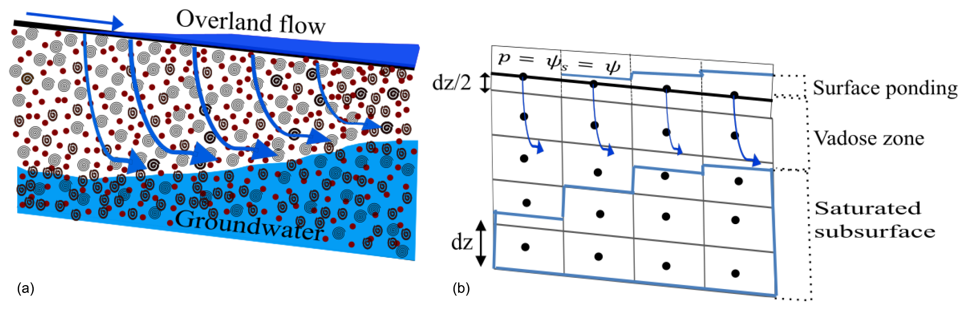
Figure 1Coupled surface and subsurface flow systems. The physical system is represented in (a), and a schematic of the overland flow boundary condition (continuity of pressure and flux at the ground surface) is in (b). The equation in Fig. 1 signifies that at the ground surface, the vertically averaged surface pressure and subsurface pressure head are equal, which is the unique overland flow boundary used by ParFlow.
Many IHMs couple subsurface and surface flows by making use of the exchange flux, qe, model. The exchange flux between the domains (the surface and the subsurface) depends on hydraulic conductivity and the gradient across some interface where indirect coupling is used (VanderKwaak, 1999; Panday and Huyakorn, 2004). The exchange flux concept gives a general formulation of a single set of coupled surface–subsurface equations. The exchange flux term, qe, may be included in the shallow overland flow continuity equation as the exchange rate term with the subsurface (Eq. 9) in a coupled system (Kollet and Maxwell, 2006).
2.4 Multiphase flow and transport equations
Most applications of the code have reflected ParFlow's core functionality as a single-phase flow solver, but there are also embedded capabilities for the multiphase flow of immiscible fluids and solute transport. Multiphase systems are distinguished from single-phase systems by the presence of one or more interfaces separating the phases, with moving boundaries between phases. The flow equations that are solved in multiphase systems in a porous medium comprise a set of mass balance and momentum equations. The equations are given by
where denotes a given phase (such as air or water). In these equations, ϕ is the porosity of the medium [-], which explains the fluid capacity of the porous medium, and for each phase, i Si(xt) is the relative saturation [-], which indicates the content of phase i in the porous medium, υi(xt) represents the Darcy velocity vector [LT−1], Qi(xt) stands for the source or sink term [T−1], pi(xt) is the average pressure , ρi(xt) is the mass density [ML−3], λi is the mobility [L3TM−1], g is the gravity vector [LT−2], and x and t represent the space vector and time, respectively. ParFlow solves for the pressures on a discrete mesh and uses a time-stepping algorithm based on a mass conservative backward Euler scheme and spatial discretization (a finite-volume method). ParFlow's multiphase flow capability has not been applied in major studies; however, this capability is also available for testing (Ashby et al., 1993; Tompson et al., 1994; Falgout et al., 1999; Maxwell et al., 2016).
The transport equations included in the ParFlow package describe mass conservation in a convective flow (no diffusion) with degradation effects and adsorption included along with extraction and injection wells (Beisman et al., 2015; Maxwell et al., 2016). The transport equation is defined as follows:
where ci,j(xt) represents the concentration fraction of contaminant [-], λi is degradation rate [T−1], Fi(xt) is the mass concentration [L3M−1], ρs(x) is the density of the solid mass [ML−3], nI is injection wells [-], is the injection rate [T−1], represents the area of the injection well [-], is the injected concentration fraction [-], nE is the extraction wells [-], is the extraction rate [T−1], is an extraction well area [-], is the number of phases, represents the number of contaminants, ci,j is the concentration of contaminant j in phase i, k is hydraulic conductivity [LT−1], is the characteristic function of an injection well region, and is the characteristic function of an extraction well region. The mass concentration term, Fi,j, is taken to be instantaneous in time and a linear function of contaminant concentration:
where Kd;j is the distribution coefficient of the component [L3M−1]. The transport–advection equation or convective flow calculation performed by ParFlow offers a choice of a first-order explicit upwind scheme or a second-order explicit Godunov scheme. The advection calculations are discretized as boundary value problems for each primary dimension over each compute cell. The discretization is a fully explicit, forward Euler, first-order accurate in time approach. The implementation of a second-order explicit Godunov scheme (second-order advection scheme) minimizes numerical dispersion and presents a more accurate computational process at these timescales than either an implicit or lower-order explicit scheme. The stability issue here is that the simulation time step is restricted via the Courant–Friedrichs–Lewy (CFL) condition, which demands that time steps are chosen as small enough to ensure that mass is not transported more than one grid cell in a single time step in order to maintain stability (Beisman, 2007).
2.5 Computational grids
An accurate numerical approximation of a set of partial differential equations is strongly dependent on the simulation grid. Integrated hydrologic models can use unstructured or structured meshes for the discretization of the governing equations. The choice of grid type to adopt is problem-specific and often a subjective choice since the same domain can be represented in many ways, but there are some clear trade-offs. For example, structured grid models, such as ParFlow, may be preferred to unstructured grid models because structured grids provide significant advantages in computational simplicity and speed, and they are amenable to efficient parallelization (Durbin, 2002; Kumar et al., 2009; Osei-Kuffuor et al., 2014). ParFlow adopts a regular, structured grid specifically for its parallel performance. There are currently two regular grid formulations included in ParFlow, an orthogonal grid and a terrain-following formulation (TFG); both allow for variable vertical discretization (thickness over an entire layer) over the domain.
2.5.1 Orthogonal grid
Orthogonal grids have many advantages, and many approaches are available to transform an irregular grid into an orthogonal grid such as conformal mapping. This mapping defines a transformed set of partial differential equations using an elliptical system with “control functions” determined in such a way that the generated grid would be either orthogonal or nearly orthogonal. However, conformal mapping may not allow flexibility in the control of the grid node distribution, which diminishes its usefulness with complex geometries (Mobley and Stewart, 1980; Haussling and Coleman, 1981; Visbal and Knight, 1982; Ryskin and Leal, 1983; Allievi and Calisal, 1992; Eca, 1996).
A Cartesian, regular, orthogonal grid formulation is implemented by default in ParFlow, though some adaptive meshing capabilities are still included in the source code. For example, layers within a simulation domain can be made to have varying thickness. Figure 2a shows the standard way that topography or any other non-rectangular domain boundaries are represented in ParFlow. The domain limits, and any other internal boundaries, can be defined using grid-independent triangulated irregular network (TIN) files that define a geometry, or a gridded indicator file can be used to define geometric elements. ParFlow uses an octree space-partitioning algorithm (a grid-based algorithm or mesh generators filled with structured grids) (Maxwell, 2013) to depict complex structure and land surface representations (e.g., topography, watershed boundaries, and different hydrologic facies) in three-dimensional space (Kollet et al., 2010). These land surface features are mapped onto the orthogonal grid, and looping structures that encompass these irregular shapes are constructed (Ashby et al., 1997). The grid cells above the ground surface are inactive (shown in Fig. 2a) and are stored in the solution vector but not included in the solution.
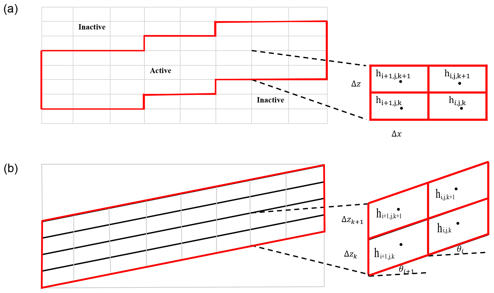
Figure 2Representation of orthogonal (a) and terrain-following (b) grid formulations and schematics of the associated finite-difference dependences (right). The i, j, and k are the x, y, and z cell indices.
2.5.2 Terrain-following grid
The inactive portion of a watershed defined with an orthogonal grid can be quite large in complex watersheds with high relief. In these cases, it is advantageous to use a grid that allows these regions to be omitted. ParFlow's structured grid conforms to the topography via transformation by the terrain-following grid formulation. This transform alters the form of Darcy's law to incorporate a topographic slope component. For example, subsurface fluxes are computed separately in both the x and y directions by making use of the terrain-following grid transform as
where qx and qy represent source or sink terms, such as fluxes, that include potential recharge flux at the ground surface [LT−1], p is the pressure head [L], K is the saturated hydraulic conductivity tensor, [LT−1], θ is the local angle [-] of topographic slope, and Sx and Sy in the x and y directions may be presented as and , respectively (Weill et al., 2009). The terrain-following grid formulation comes in handy when solving coupled surface and subsurface flows (Maxwell, 2013). The terrain-following grid formulation uses the same surface slopes specified for overland flow to transform the grid, whereas the slopes specified in the orthogonal grid are only used for 2-D overland flow routing and do not impact the subsurface formulation (see Fig. 2). Note that TIN files can still be used to deactivate portions of the transformed domain.
The core of the ParFlow code is its library of numerical solvers. As noted above, in most cases, the temporal discretization of the governing equations uses an implicit (backward Euler) scheme with cell-centered finite differences in spatial dimensions. Different components of this solution framework have been developed for the various operational modes of ParFlow including an inexact Newton–Krylov nonlinear solver (Sect. 3.1), a multigrid algorithm (Sect. 3.2), and a multigrid-preconditioned conjugate gradient (MGCG) solver in (Sect. 3.3). The conditions, requirements, and constraints on the solvers depend on the specifics of the problem being solved, and some solvers tend to be more efficient (faster overall convergence) than others for a given problem. The core structure of these solvers and some of their implementation details are given below, with an emphasis on the main concepts behind each solver.
3.1 Newton–Krylov solver for variably saturated flow
The cell-centered fully implicit discretization scheme applied to the Richards equation leads to a set of coupled discrete nonlinear equations that need to be solved at each time step, and, for variably saturated subsurface flow, ParFlow does this with the inexact Newton–Krylov method implemented in the KINSOL package (Hindmarsh et al., 2005; Collier et al., 2015). Newton–Krylov methods were initially utilized in the context of partial differential equations by Brown and Saad (1990). In the approach, a coupled nonlinear system as a result of discretization of the partial differential equation is solved iteratively. Within each iteration, the nonlinear system is linearized via a Taylor expansion. After linearization, an iterative Krylov method is used to solve the resulting linear Jacobian system (Woodward, 1998; Osei-Kuffuor et al., 2014). For variably saturated subsurface flow, ParFlow uses the GMRES Krylov method (Saad and Schultz, 1986). Figure 3 is a flowchart of the solution technique ParFlow uses to provide approximate solutions to systems of nonlinear equations.
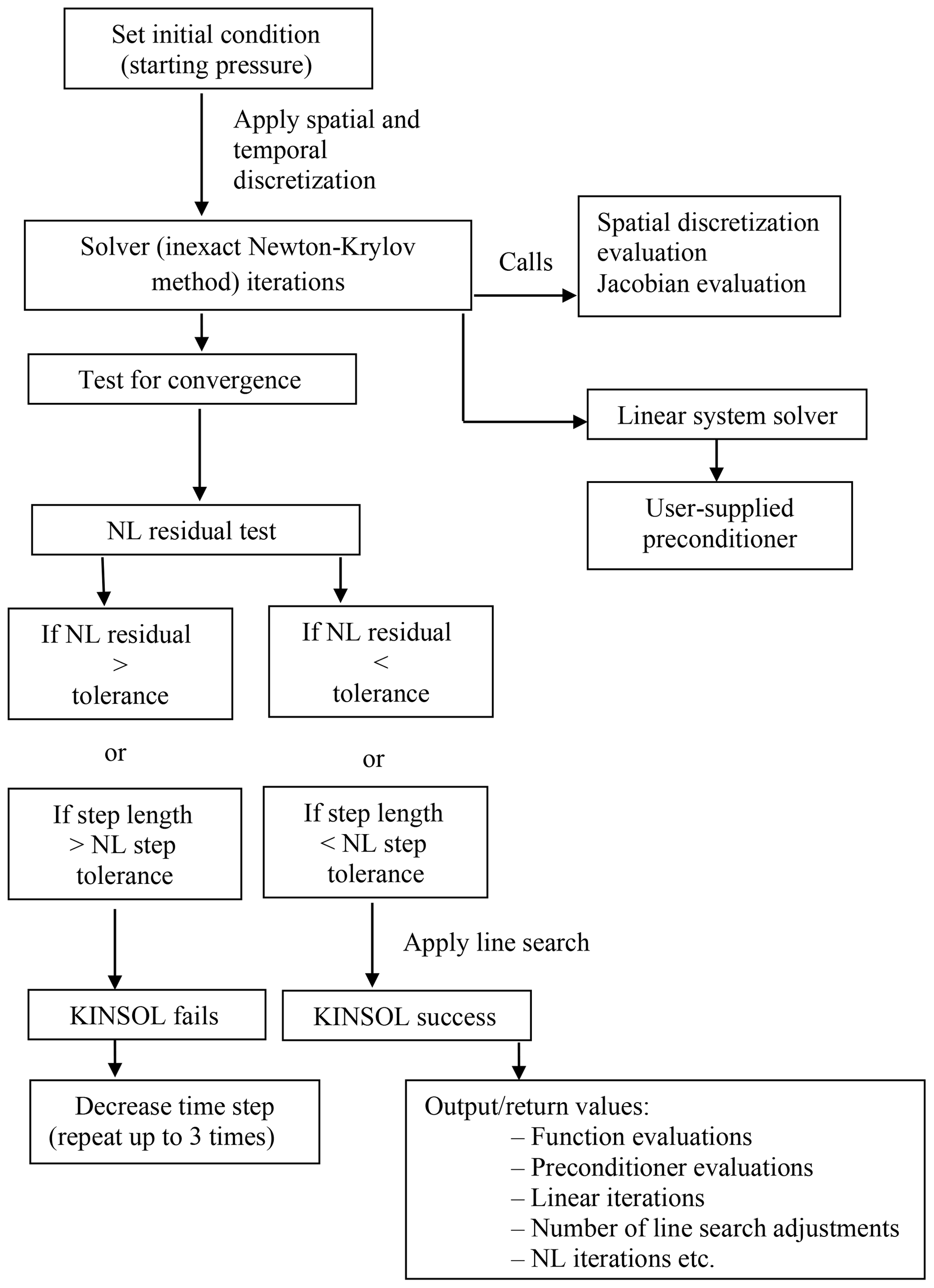
The benefit of this Newton–Krylov method is that the Krylov linear solver requires only matrix–vector products. Because the system matrix is the Jacobian of the nonlinear function, these matrix–vector products may be approximated by taking directional derivatives of the nonlinear function in the direction of the vector to be multiplied. This approximation is the main advantage of the Newton–Krylov approach as it removes the requirement for matrix entries in the linear solver. An inexact Newton method is derived from a Newton method by using an approximate linear solver at each nonlinear iteration, as is done in the Newton–Krylov method (Dembo and Eisenstat, 1982; Dennis Jr. and Schabel, 1996). This approach takes advantage of the fact that when the nonlinear system is far from converged, the linear model used to update the solution is a poor approximation. Thus, the convergence criteria for an early linear system solver are relaxed. The tolerance required for the solution of the linear system is decreased as the nonlinear function residuals approach zero. The convergence rate of the resulting nonlinear solver can be linear or quadratic, depending on the algorithm used. Through the KINSOL package, ParFlow can either use a constant tolerance factor or ones from Eisenstat and Walker (1996). Krylov methods can be very robust, but they can be slow to converge. As a result, it is often necessary to implement a preconditioner, or accelerator, for these solvers.
3.2 Multigrid solver
Multigrid (MG) methods constitute a class of techniques or algorithms for solving differential equations (system of equations) using a hierarchy of discretization (Briggs et al., 2000). Multigrid algorithms are applied primarily to solve linear and nonlinear boundary value problems and can be used as either preconditioners or solvers. The most efficient method for preconditioning linear systems in ParFlow is the ParFlow Multigrid (PFMG) algorithm (Ashby and Falgout, 1996; Jones and Woodward, 2001). Multigrid algorithms arise from the discretization of elliptic partial differential equations (Briggs et al., 2000) and, in ideal cases, have convergence rates that do not depend on the problem size. In these cases, the number of iterations remains constant even as problem sizes grow large. Thus, the algorithm is algorithmically scalable. However, it may take longer to evaluate each iteration as problem sizes increase. As a result, ParFlow utilizes the highly efficient implementation of the PFMG in the hypre library (Falgout and Yang, 2002).
For variably saturated subsurface flow, ParFlow uses the Newton–Krylov method coupled with a multigrid preconditioner to accurately solve for the water pressure (hydraulic head) in the subsurface and diagnoses the saturation field (which is used in determining the water table) (Woodward, 1998; Jones and Woodward, 2000, 2001; Kollet et al., 2010). The water table is calculated for computational cells having hydraulic heads above the bottom of the cells. Generally, a cell is saturated if the hydraulic head in the cell is above the node elevation (cell center), or the cell is unsaturated if the hydraulic head in the cell is below the node elevation. For saturated flow, ParFlow uses the conjugate gradient method also coupled with a multigrid method. It is important to note that subsurface flow systems are usually much larger radially than they are thick, so it is common for computational grids to have highly anisotropic cell aspect ratios to balance the lateral and vertical discretization. Combined with anisotropy in the permeability field, these high aspect ratios produce numerical anisotropy in the problem, which can cause the multigrid algorithms to converge slowly (Jones and Woodward, 2001). To correct this problem, a semi-coarsening strategy or algorithm is employed, whereby the grid is coarsened in one direction at a time. The direction chosen is the one with the smallest grid spacing, i.e., the tightest coupling. In an instance in which more than one direction has the same minimum spacing, then the algorithm chooses the direction in the order of x, followed by y, and then in z. To decide on how and when to terminate the coarsening algorithm, Ashby and Falgout (1996) determined that a semi-coarsening down to a grid is ideal for groundwater problems.
3.3 Multigrid-preconditioned conjugate gradient (MGCG)
ParFlow uses the multigrid-preconditioned conjugate gradient (CG) solver to solve the groundwater equations under steady-state and fully saturated flow conditions (Ashby and Falgout, 1996). These problems are symmetric and positive definite, two properties the CG method was designed to target. While CG lends itself to efficient implementations, the number of iterations required to solve a system that results from the discretization of the saturated flow equation increases as the problem size grows. The PFMG algorithm is used as a preconditioner to combat this growth and results in an algorithm for which the number of iterations required to solve the system grows only minimally. See Ashby and Falgout (1996) for a detailed description of these solvers and the parallel implementation of the multigrid-preconditioned CG method in ParFlow (Gasper et al., 2014; Osei-Kuffuor et al., 2014).
3.4 Preconditioned Newton–Krylov for coupled subsurface–surface flows
As discussed above, coupling between subsurface and surface or overland flow in ParFlow is activated by specifying an overland boundary condition at the top surface of the computational domain, but this mode of coupling allows for activation and deactivation of the overland boundary condition during simulations in which ponding or drying occurs. Thus, surface–subsurface coupling can occur anywhere in the domain during a simulation, and it can change dynamically during the simulation. Overland flow may occur by the Dunne or Horton mechanism depending on local dynamics. Overland flow routing is enabled when the subsurface cells are fully saturated. In ParFlow the coupling between the subsurface and surface flows is handled implicitly. ParFlow solves this implicit system with the inexact Newton–Krylov method described above. However, in this case, the preconditioning matrix is adjusted to include terms from the surface coupling. In the standard saturated or variably saturated case, the multigrid method is given the linear system matrix, or a symmetric version, resulting from the discretization of the subsurface model. Because ParFlow uses a structured mesh, these matrices have a defined structure, making their evaluation and the application of a multigrid straightforward. Due to varying topographic height of the surface boundary, where the surface coupling is enforced, the surface effects add nonstructured entries in the linear system matrices. These entries increase the complexity of the matrix entry evaluations and reduce the effectiveness of the multigrid preconditioner. In this case, the matrix–vector products are most effectively performed through the computation of the linear system entries rather than the finite-difference approximation to the directional derivative. For the preconditioning, surface couplings are only included if they model flow between cells at the same vertical height, i.e., in situations in which overland flow boundary conditions are imposed or activated. This restriction maintains the structured property of the preconditioning matrix while still including much of the surface coupling in the preconditioner. Both these adjustments led to considerable speedup in coupled simulations (Osei-Kuffuor et al., 2014).
Scaling efficiency metrics offer a quantitative method for evaluating the performance of any parallel model. Good scaling generally means that the efficiency of the code is maintained as the solution of the system of equations is distributed onto more processors or as the problem resolution is refined and processing resources are added. Scalability can depend on the problem size, the processor number, the computing environment, and the inherent capabilities of the computational platform used, e.g., the choice of a solver. The performance of ParFlow (or any parallel code) is typically determined through weak and strong scaling (Gustafson, 1988). Weak scaling involves the measurement of the code's efficiency in solving problems of increasing size (i.e., it describes how the solution time changes with a change in the number of processors for a fixed problem size per processor). In weak scaling, the simulation time should remain constant, as the size of the problem and number of processing elements grow such that the same amount of work is conducted on each processing element. Following Gustafson (1988), scaled parallel efficiency is given by
where E(np) denotes parallel efficiency, and T represents the runtime as a function of the problem size n, which is spread across several processors, p. Parallel code is said to be perfectly efficient if , and the efficiency decreases as E(np) approaches 0. Generally, parallel efficiency decreases with increasing processor number as communication overhead between nodes and/or processors becomes the limiting factor.
Strong scaling describes the measurement of how much the simulation or solution time changes with the number of processors for a given problem of fixed total size (Amdahl, 1967). In strong scaling, a fixed size task is solved on a growing number of processors, and the associated time needed for the model to compute the solution is determined (Woodward, 1998; Jones and Woodward, 2000). If the computational time decreases linearly with the processor number, a perfect parallel efficiency, (E=1), results. The value of E is determined using Eq. (19). ParFlow has been shown to have excellent parallel performance efficiency, even for large problem sizes and processor counts (see Table 1) (Ashby and Falgout, 1996; Kollet and Maxwell, 2006). In situations in which ParFlow works in conjunction with or coupled to other subsurface, land surface, or atmospheric models (see Sect. 5), i.e., increased computational complexity by adding different components or processes, improved computational time may not only depend on ParFlow. The computational cost of such an integrated model is extremely difficult to predict because of the nonlinear nature of the system. The solution time may depend on a number of factors including the number of degrees of freedom, the heterogeneity of the parameters, and which processes are active (e.g., snow accumulation compared to nonlinear snowmelt processes in a land surface model or the switching on or off of the overland flow routing in ParFlow). The only way to know how fast a specific problem will run is to try that problem. Many of the studies presented in Table 1 include computational times for problems with different complexities when ParFlow was used. In a scaling study with ParFlow, Maxwell (2013) examined the relative performance of preconditioning the coupled variably saturated subsurface and surface flow system with the symmetric portion or full matrix for the system. Both options use ParFlow's multigrid preconditioner. Solver performance was demonstrated by combining the analytical Jacobian and the nonsymmetric linear preconditioner. The study showed that the nonsymmetric linear preconditioner presents faster computational times and efficient scaling. A section of the study results is reproduced in Table 1, in addition to other scaling studies demonstrating ParFlow's parallel efficiency. This trade-off was also examined in Jones and Woodward (2000).
Table 1Details for the various scaling studies conducted using ParFlow.
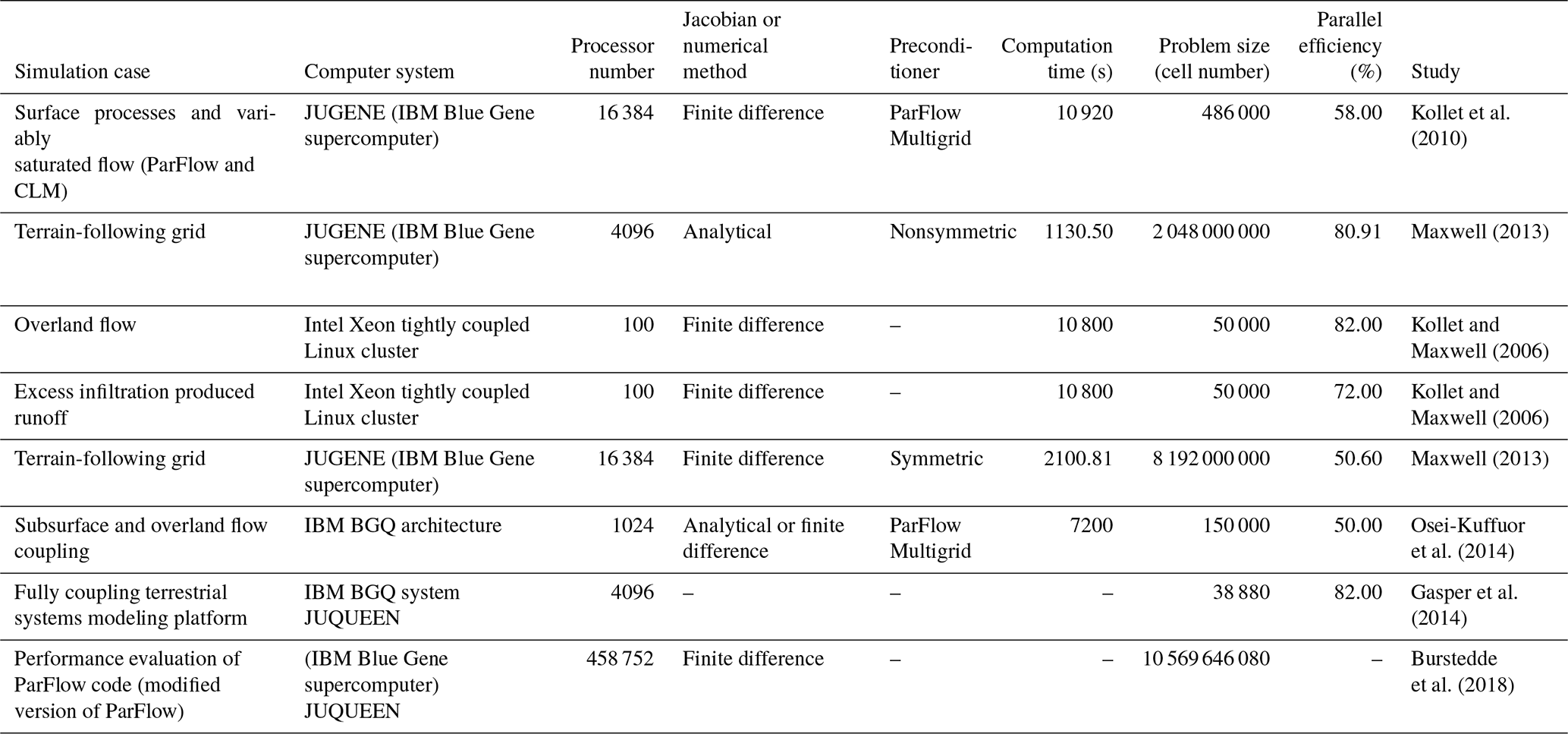
A dash (–) indicates that information was not provided by the appropriate study.
It is worth noting that large and/or complex problem sizes (e.g., simulating a large heterogenous domain size with over 8.1 billion unknowns) will always take time to solve directly, but the approach for setting up a problem depends on the specific problem being modeled. Even for one specific kind of model there may be multiple workflows, and how to model such complexity becomes the sole responsibility of the modeler. The studies involving ParFlow outlined in Table 1 provide a wealth of knowledge regarding domain setup for problems of different complexities. Since these are all specific applications, the information will likely be very useful to modelers trying to build a new domain during the setup and planning phases.
Different integrated models, including atmospheric or weather prediction models (e.g., Weather Research Forecasting model, Advanced Regional Prediction System, Consortium for Small-Scale Modeling), land surface models (e.g., Common Land Model, Noah Land Surface Model), and a subsurface model (e.g., CrunchFlow), have been coupled with ParFlow to simulate a variety of coupled earth system effects (see Fig. 4a). Coupling between ParFlow and other integrated models was performed to better understand the physical processes that occur at the interfaces between the deeper subsurface and ground surface, as well as between the ground surface and the atmosphere. None of the individual models can achieve this on their own because ParFlow cannot account for land surface processes (e.g., evaporation), and atmospheric and land surface models generally do not simulate deeper subsurface flows (Ren and Xue, 2004; Chow et al., 2006; Beisman, 2007; Maxwell et al., 2007; Shi et al., 2014). Model coupling can be achieved either via “offline coupling”, whereby models involved in the coupling process are run sequentially and interactions between them are one-way (i.e., information is only transmitted from one model to the other), or “online” whereby they interact and feedback mechanisms among components are represented (Meehl et al., 2005; Valcke et al., 2009). Each of the coupled models uses its own solver for the physical system it is solving, and then information is passed between the models. As long as each model exhibits good parallel performance, this approach still allows for simulations at very high resolution, with a large number of processes (Beven, 2004; Ferguson and Maxwell, 2010; Shen and Phanikumar, 2010; Shi et al., 2014). This section focuses on the major couplings between ParFlow and other codes. We point out specific functions of the individual models as stand-alone codes that are relevant to the coupling process. In addition, information about the role or contribution of each model at the coupling interface (see Fig. 4b) that connects with ParFlow is presented (Fig. 5 shows the communication network of the coupled models). We discuss couplings between ParFlow and its land surface model (a modified version of the original Common Land Model introduced by Dai et al. 2003), the Consortium for Small-Scale Modeling (COSMO), the Weather Research Forecasting model, the Advanced Regional Prediction System, and CrunchFlow in Sect. 5.1, 5.2, 5.3, 5.4, and 5.5, respectively.
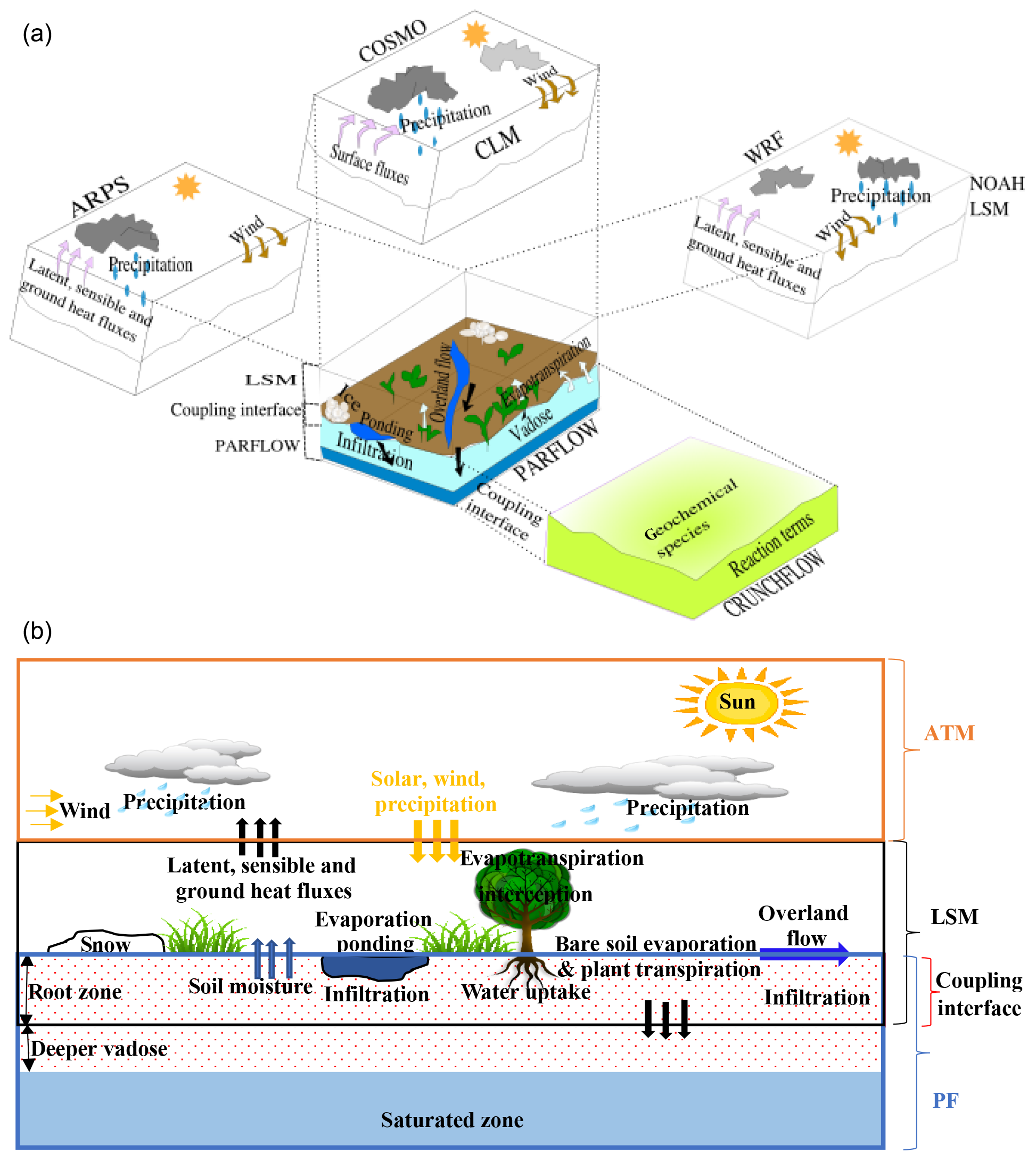
Figure 4(a) A pictorial description of the relevant physical environmental features and model coupling. CLM represents the Community Land Model, a stand-alone land surface model (LSM) via which ParFlow couples to COSMO. The modified version of CLM by Dai et al. (2003) is not shown because it is a module only for ParFlow, not really a stand-alone LSM any longer. The core model (ParFlow) always solves the variably saturated 3-D groundwater flow problem, but the various couplings add additional capabilities. (b) Schematic showing information transmission at the coupling interface. PF, LSM, and ATM indicate the portions of the physical system simulated by ParFlow, land surface models, and atmospheric models, respectively. The downward and upward arrows indicate the directions of information transmission between adjacent models. Note: coupling between ParFlow and CrunchFlow (not shown) occurs within the subsurface.
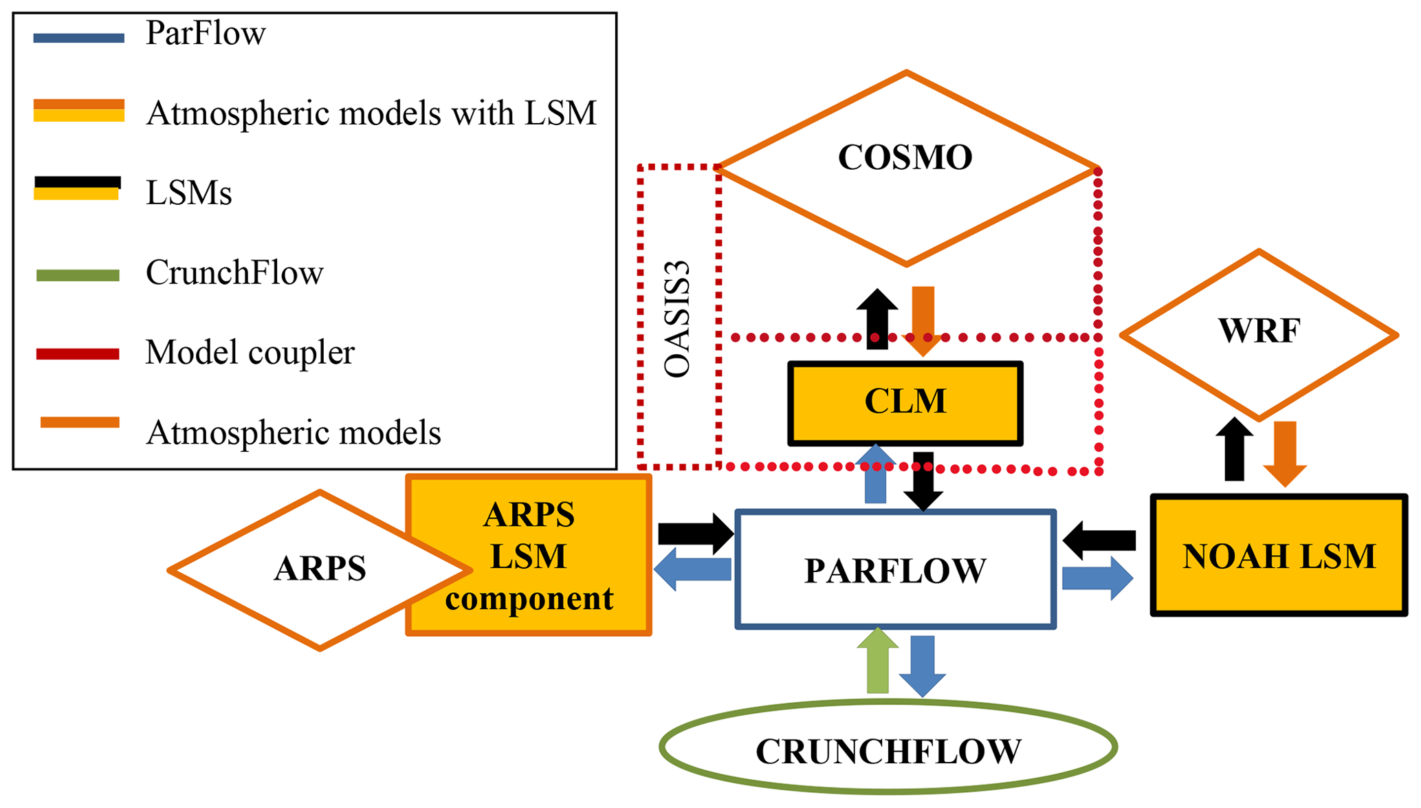
Figure 5Schematic of the communication structure of the coupled models. Note: CLM represents the stand-alone Community Land Model. The modified version of the Common Land Model by Dai et al. (2003) is not shown here because it is a module only for ParFlow, not really a stand-alone LSM any longer.
5.1 ParFlow–Common Land Model (PF.CLM)
The Common Land Model (CLM) is a land surface model designed to complete land–water–energy balance at the land surface (Dai et al., 2003). CLM parameterizes the moisture, energy, and momentum balances at the land surface and includes a variety of customizable land surface characteristics and modules, including land surface type (land cover type, soil texture, and soil color), vegetation and soil properties (e.g., canopy roughness, zero-plane displacement, leaf dimension, rooting depths, specific heat capacity of dry soil, thermal conductivity of dry soil, porosity), optical properties (e.g., albedos of thick canopy), and physiological properties related to the functioning of the photosynthesis–conductance model (e.g., green leaf area, dead leaf, and stem area indices). A combination of numerical schemes is employed to solve the governing equations. CLM uses a time integration scheme that proceeds through a split-hybrid approach, in which the solution procedure is split into “energy balance” and “water balance” phases in a very modularized structure (Mikkelson et al., 2013; Steiner et al., 2005, 2009). The CLM described here and as incorporated in ParFlow is a modified version of the original CLM introduced by Dai et al. (2003), though the original version was coupled to ParFlow in previous model applications (e.g., Maxwell and Miller, 2005). The current coupled model, PF.CLM, consists of ParFlow incorporated with a land surface model (Jefferson et al., 2015, 2017; Jefferson and Maxwell, 2015). The modified CLM is composed of a series of land surface modules that are called as a subroutine within ParFlow to compute energy and water fluxes (e.g., evaporation and transpiration) to and out of the soil. For example, the modified CLM computes the bare ground surface evaporative flux, Egr, as
where β (dimensionless) denotes the soil resistance factor, ρa represents air density [ML−3], u∗ represents friction velocity [LT−1], and q∗ (dimensionless) stands for the humidity scaling parameter (Jefferson and Maxwell, 2015). Evapotranspiration for vegetated land surface, Eveg, is computed as
where rb is the air density boundary resistance factor [LT−1], qsat (dimensionless) is saturated humidity at the land surface, and qaf (dimensionless) is the canopy humidity. The combination of qsat and qaf forms the potential evapotranspiration. The potential evapotranspiration is divided into transpiration Rpp,dry (dimensionless), which depends on the dry fraction of the canopy, and evaporation from foliage covered by water Lw (dimensionless). LSAI (dimensionless) is the summation of the leaf and stem area indices that estimates the total surface from which evaporation can occur. A detailed description of the equations PF.CLM uses can be found in Jefferson et al. (2015, 2017) and Jefferson and Maxwell (2015).
PF.CLM simulates variably saturated subsurface flow, surface or overland flow, and aboveground processes. PF.CLM was developed prior to the current Community Land Model (see Sect. 5.2), and the module structure of the current and early versions are different. PF.CLM has been updated over the years to improve its capabilities. PF.CLM was first done in the early 2000s as an undiversified, a column proof-of-concept model, whereby data or a message was transmitted between the coupled models via input/output files (Maxwell and Miller, 2005). Later, PF.CLM was presented in a distributed or diversified approach with a parallel input/output file structure wherein CLM is called as a set sequence of steps within ParFlow (Kollet and Maxwell, 2008a). These modifications, for example, were done to incorporate subsurface pressure values from ParFlow into chosen computations (Jefferson and Maxwell, 2015). These, to some extent, differentiate the modified version (PF.CLM) from the original CLM by Dai et al. (2003). Within the coupled PF.CLM, ParFlow solves the governing equations for overland and subsurface flow systems, and the CLM modules add the energy balance and mass fluxes from the soil, canopy, and root zone that can occur (i.e., interception, evapotranspiration, etc.) (Jefferson and Maxwell, 2015).
At the coupling interface where the models overlap and undergo online communication (Fig. 4b), ParFlow calculates and passes soil moisture and pressure heads of the subsurface to CLM, and CLM calculates and transmits transpiration from plants, canopy and ground surface evaporation, snow accumulation and melt, and infiltration from precipitation to ParFlow (Ferguson et al., 2016). In short, CLM does all canopy water balances and snow, but once the water through falls to the ground or snow melts, ParFlow takes over and estimates the water balances via the nonlinear Richards equation. The coupled model, PF.CLM, has been shown to more accurately predict root-depth soil moisture compared to the uncoupled model, i.e., the stand-alone land surface model (CLM), with capability to compute near-surface soil moisture. This increased accuracy results from the coupling of soil saturations determined by ParFlow and their impacts on other processes including runoff and infiltration (Kollet, 2009; Shrestha et al., 2014; Gebler et al., 2015; Gilbert and Maxwell, 2017). For example, Maxwell and Miller (2005) found that simulations of deeper soil saturation (more than 40 cm) vary between PF.CLM and uncoupled models, with PF.CLM simulations closely matching the observed data. Table 2 contains summaries of studies conducted with ParFlow coupled to either the original version of CLM by Dai et al. (2003) or the modified CLM (ParFlow with a land surface model).
Table 2Selected coupling studies involving the application of ParFlow and atmospheric, land surface, and subsurface models.
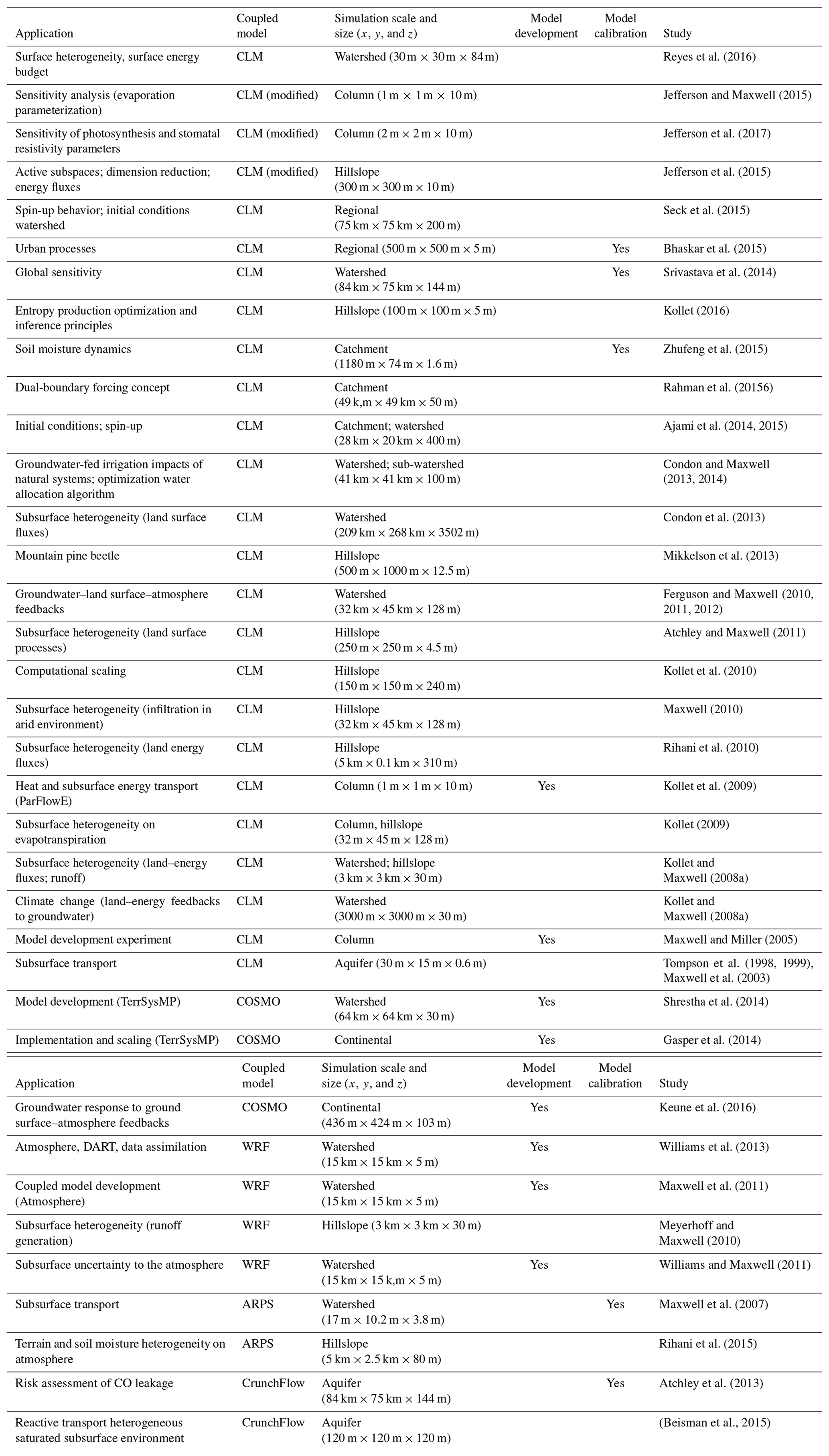
“CLM” indicates that coupling with ParFlow was by the original Common Land
Model or Community Land Model. “CLM (modified)” indicates that the modified
version of
the Common Land Model by Dai et al. (2003) was a module for ParFlow.
ParFlowE–Common Land Model (ParFlowE[CLM])
It is well established that ParFlow in conjunction with CLM performs well in estimating all canopy water and subsurface water balances (Maxwell and Miller, 2005; Mikkelson et al., 2013; Ferguson et al., 2016). ParFlow, as a component of the coupled model, has been modified into a new parallel numerical model, ParFlowE, to incorporate the more complete heat equation coupled to variably saturated flow. ParFlowE simulates the coupling of terrestrial hydrologic and energy cycles, i.e., coupled moisture, heat, and vapor transport in the subsurface. ParFlowE is based on the original version of ParFlow, having identical solution schemes and a coupling approach as CLM. A coupled three-dimensional subsurface heat transport equation is implemented in ParFlowE using a cell-centered finite-difference scheme in space and an implicit backward Euler differencing scheme in time. However, the solution algorithm employed in ParFlow is fully exploited in ParFlowE wherein the solution vector of the Newton–Krylov method was extended to two dimensions (Kollet et al., 2009). In some integrated and climate models, the convection term of subsurface heat flux and the effect of soil moisture on energy transport is neglected due to simplified parameterizations and computational limitations. However, both convection and conduction terms are considered in ParFlowE (Khorsandi et al., 2014). In ParFlowE, functional relationships (i.e., equations of state) are performed to relate density and viscosity to temperature and pressure, as well as thermal conductivity to saturation. That is, modeling thermal flows by relating these parameterizations in simulating heat flow is an essential component of ParFlowE. In coupling between ParFlowE and CLM, ParFlowE[CLM], the one-dimensional subsurface heat transport in the CLM, is replaced by the three-dimensional heat transport equation including the process of convection of ParFlowE. CLM computes the mass and energy balances at the ground surface that lead to moisture fluxes and passes these fluxes to the subsurface moisture algorithm of ParFlowE[CLM]. These fluxes are used to compute subsurface moisture and temperature fields, which are then passed back to the CLM.
5.2 ParFlow in the Terrestrial Systems Modeling Platform, TerrSysMP
ParFlow is part of the Terrestrial System Modeling Platform TerrSysMP, which comprises the nonhydrostatic fully compressible limited-area atmospheric prediction model, COSMO, designed for both operational numerical weather prediction and various scientific applications on the meso-β (horizontal scales of 20–200 km) and meso-γ (horizontal scales of 2–20 km) (Duniec and Mazur, 2011; Levis and Jaeger, 2011; Bettems et al., 2015), and the Community Land Model version 3.5 (CLM3.5). Currently, it is used in direct simulations of severe weather events triggered by deep moist convection, including intense mesoscale convective complexes, prefrontal squall-line storms, supercell thunderstorms, and heavy snowfall from wintertime mesocyclones. COSMO solves nonhydrostatic, fully compressible hydro-thermodynamical equations in advection form using the traditional finite-difference method (Vogel et al., 2009; Mironov et al., 2010; Baldauf et al., 2011; Wagner et al., 2016).
An online coupling between ParFlow and the COSMO model is performed via CLM3.5 (Gasper et al., 2014; Shrestha et al., 2014; Keune et al., 2016). Similar to the Common Land Model (by Dai et al., 2003), the CLM3.5 module accounts for surface moisture, carbon, and energy fluxes between the shallow or near-surface soil (discretized or specified top soil layer), snow, and the atmosphere (Oleson et al., 2008). The model components of a fully coupled system consisting of COSMO, CLM3.5, and ParFlow are assembled by making use of the multiple–executable approach (e.g., with the OASIS3–MCT model coupler). The OASIS3–MCT coupler employs communication strategies based on the message passing interface standards MPI1/MPI2 and the Project for Integrated Earth System Modeling, PRISM, Model Interface Library (PSMILe) for parallel communication of two-dimensional arrays between the OASIS3–MCT coupler and the coupling models (Valcke et al., 2012; Valcke, 2013). The OASIS3–MCT specifies the series of coupling, frequency of the couplings, the coupling fields, the spatial grid of the coupling fields, the transformation type of the (two-dimensional) coupled fields, and simulation time management and integration.
At the coupling interface, the OASIS3–MCT interface interchanges the atmospheric forcing terms and the surface fluxes in serial mode. The lowest level and current time step of the atmospheric state of COSMO is used as the forcing term for CLM3.5. CLM3.5 then computes and returns the surface energy and momentum fluxes, outgoing longwave radiation, and albedo to COSMO (Baldauf et al., 2011). The air temperature, wind speed, specific humidity, convective and grid-scale precipitation, pressure, incoming shortwave (direct and diffuse) and longwave radiation, and measurement height are sent from COSMO to CLM3.5. In CLM3.5, a mosaic tiling approach may be used to represent the subgrid-scale variability of land surface characteristics, which considers a certain number of patches or tiles within a grid cell. The surface fluxes and surface state variables are first calculated for each tile and then spatially averaged over the whole grid cell (Shrestha et al., 2014). As with PF.CLM3.5, the one-dimensional soil column moisture predicted by CLM3.5 gets replaced by ParFlow's variably saturated flow solver, so ParFlow is responsible for all calculations relating to soil moisture redistribution and groundwater flow. Within the OASIS3–MCT ParFlow sends the calculated pressure and relative saturation for the coupled region soil layers to CLM3.5. CLM3.5 also transmits depth-differentiated source and sink terms for soil moisture including soil moisture flux, e.g., precipitation, and soil evapotranspiration for the coupled region soil layers to ParFlow. Applications of TerrSysMP in fully coupled mode from saturated subsurface across the ground surface into the atmosphere include a study on the impact of groundwater on the European heat wave of 2003 and the influence of anthropogenic water use on the robustness of the continental sink for atmospheric moisture content (Keune et al., 2016).
5.3 ParFlow–Weather Research and Forecasting models (PF.WRF)
The Weather Research and Forecasting (WRF) model is a mesoscale numerical weather prediction system designed to be flexible and efficient in a massively parallel computing architecture. WRF is a widely used model that provides a common framework for idealized dynamical studies, full-physics numerical weather prediction, air-quality simulations, and regional climate simulations (Michalakes et al., 1999, 2001; Skamarock et al., 2005). The model contains numerous mesoscale physics options such as microphysics parameterizations (including explicitly resolved water vapor, cloud, and precipitation processes), surface layer physics, shortwave radiation, longwave radiation, land surface, planetary boundary layer, data assimilation, and other physics and dynamics alternatives suitable for both large-eddy and global-scale simulations. Similar to COSMO, the WRF model is a fully compressible, conservative-form, nonhydrostatic atmospheric model that uses time-splitting integration techniques (discussed below) to efficiently integrate the Euler equations (Skamarock and Klemp, 2007).
The online ParFlow WRF coupling (PF.WRF) extends the WRF platform down to the bedrock by including highly resolved three-dimensional groundwater and variably saturated shallow or deep vadose zone flows, as well as a fully integrated lateral flow above the ground surface (Molders and Ruhaak, 2002; Seuffert et al., 2002; Anyah et al., 2008; Maxwell et al., 2011). The land surface model portion that links ParFlow to WRF is supplied by WRF through its land surface component, the Noah Land Surface Model (Ek et al., 2003); the stand-alone version of WRF has no explicit model of subsurface flow. Energy and moisture fluxes from the land surface are transmitted between the two models via the Noah LSM that accounts for the coupling interface and is conceptually identical to the coupling in PF–COSMO. The three-dimensional variably saturated subsurface and two-dimensional overland flow equations, and the three-dimensional atmospheric equations given by ParFlow and WRF, are simultaneously solved by the individual model solvers. Land surface processes, such as evapotranspiration, are determined in the Noah LSM as a function of potential evaporation and vegetation fraction. This effect is calculated with the formulation
where E(x) stands for the rate of soil evapotranspiration (length per unit time), fx represents empirical coefficient, favg denotes vegetation fraction, and Epot is potential evaporation, determined depending on atmospheric conditions from the WRF boundary layer parameterization (Ek et al., 2003). The vegetation fraction is zero over bare soils (i.e., only soil evaporation), so Eq. (22) becomes
The quantity F is parameterized as follows:
where ϕ is the porosity of the medium, and Sw and Sres are relative saturation and residual saturation, respectively, from the van Genuchten relationships (van Genuchten, 1980; Williams and Maxwell, 2011). Basically, F refers to the parameterization of the interrelationship between evaporation and near-ground soil water content and provides one of the connections between Noah LSM, ParFlow, and thus WRF.
In the presence of a vegetation layer, plant transpiration (length per unit time) is determined as follows:
where Cplant(−) represents a constant coefficient between 0 and 1, which depends on vegetation species, and the G(z) function represents soil moisture, which provides other connections between the coupled models (i.e., ParFlow, Noah, and WRF). The solution procedure of PF.WRF uses an operator-splitting approach in which both model components use the same time step. WRF soil moisture information, including runoff, surface ponding effects, and unsaturated and saturated flow, which includes an explicitly resolved water table, is calculated and sent directly to the Noah LSM within WRF by ParFlow and utilized by the Noah LSM in the next time step. WRF supplies ParFlow with evapotranspiration rates and precipitation via the Noah LSM (Jiang et al., 2009). The interdependence between the energy and land balance of the subsurface, ground surface, and lower atmosphere can fully be studied with this coupling approach. The coupled PF.WRF via the Noah LSM has been used to simulate explicit water storage and precipitation within basins, surface runoff, and the land–atmosphere feedbacks and wind patterns as a result of subsurface heterogeneity (Maxwell et al., 2011; Williams and Maxwell, 2011). Studies with the coupled model PF.WRF are highlighted in Table 2.
5.4 ParFlow–Advanced Regional Prediction System (PF.ARPS)
The Advanced Regional Prediction System (ARPS) is composed of a parallel mesoscale atmospheric model created to explicitly predict convective storms and weather systems. The ARPS platform aids in effectively investigating the changes and predictability of storm-scale weather in both idealized and more realistic settings. The model deals with the three-dimensional, fully compressible, nonhydrostatic, spatially filtered Navier–Stokes equations (Rihani et al., 2015). The governing equations include the conservation of momentum, mass, water, heat or thermodynamics, turbulent kinetic energy, and the equation of state of moist air by making use of a terrain-following curvilinear coordinate system (Xue et al., 2000). The governing equations presented in a coordinate system with z as the vertical coordinate are given as follows.
Equations (26) to (29) are momentum, continuity, thermodynamics, and the equation of state, respectively. The material (total) derivative d∕dt is defined as
The variables v, ρ, T, P, g, F, and Q in Eqs. (26) to (29) represent velocity [LT−1], density [ML−3], temperature [K], pressure , gravity [LT−2], frictional force [MLT−2], and the diabatic heat source , respectively (Xu et al., 1991). The ARPS model employs a high-order monotonic advection technique for scalar transport and fourth-order advection for other variables, e.g., mass density and mass mixing ratio. A split-explicit time advancement scheme is utilized with leapfrog on the large time steps, and an explicit and implicit scheme for the smaller time steps is used to inculcate the acoustic terms in the equations (Rihani et al., 2015).
The PF.ARPS forms a fully coupled model that simulates spatial variations in aboveground processes and feedbacks, forced by physical processes in the atmosphere and below the ground surface. In the online coupling process, the ARPS land surface model forms the interface between ParFlow and ARPS to transmit information (i.e., surface moisture fluxes) between the coupled models. ParFlow, as a component of the coupled model, replaces the subsurface hydrology in the ARPS land surface model. Thus, ARPS is integrated into ParFlow as a subroutine to create a numerical overlay at the coupling interphase (specified layers of soil within the land surface model in ARPS) with the same number of soil layers at the ground surface within ParFlow. The solution approach employed is an operator splitting that allows ParFlow to match the ARPS internal time steps. ParFlow calculates the subsurface moisture field at each time step of a simulation and passes the information to the ARPS land surface model, which is used in each subsequent time step. At the beginning of each time step, the surface fluxes from ARPS that are important to ParFlow include the evapotranspiration rate and spatially variable precipitation (Maxwell et al., 2007). PF.ARPS has been applied to investigate the effects of soil moisture heterogeneity on atmospheric boundary layer processes. PF.ARPS keeps a realistic soil moisture that is topographically driven and shows a spatiotemporal relationship between water depth, land surface, and lower atmospheric variables (Maxwell et al., 2007; Rihani et al., 2015). A summary of current studies involving PF.ARPS is included in Table 2.
5.5 ParFlow–CrunchFlow (ParCrunchFlow)
CrunchFlow is a software package developed to simulate multicomponent multidimensional reactive flow and transport in porous and/or fluid media (Steefel, 2009). Systems of chemical reactions that can be solved by the code include kinetically controlled homogenous and heterogeneous mineral dissolution reactions, equilibrium-controlled homogeneous reactions, thermodynamically controlled reactions, and biologically mediated reactions (Steefel and Lasaga, 1994; Steefel and Yabusaki, 1996). In CrunchFlow, discretization of the governing coupled partial differential equations that connect subsurface kinetic reactions and multicomponent equilibrium, flow, and solute transport is based on finite volume (Li et al., 2007, 2010). The coupling of reactions and transport in CrunchFlow that are available at runtimes is performed using two approaches. These are briefly discussed below.
The first is a global implicit or one-step method approach based on a backwards Euler time discretization, with a global solution of the coupled reactive transport equations using Newton's method. This global implicit scheme solves the transport and reaction terms simultaneously (up to two-dimensional) (Kirkner and Reeves, 1988; Steefel, 2009). The second is a time or operator splitting of the reaction and transport terms, which is based on an explicit forward Euler method: the sequential noniterative approach, SNIA (in which the transport and reaction terms are solved) (Steefel and Van Cappellen, 1990; Navarre-Sitchler et al., 2011). The stability criterion associated with the explicit approach is that the simulation time step is restricted via the Courant–Friedrichs–Lewy (CFL) condition, under the circumstance that the transportation of mass does not occur over multiple grid cells, but a single grid cell in a time step. Thus, a small time step must be used to ensure this condition holds. This small step size may lead to simulations that will demand much more time to solve Beisman (2007), so more processors are used in order to decrease the processor workload and decrease the solution time of the simulation. The coupling of fully saturated flow to the reactive transport calculations and coupling between a partially saturated flow and transport (flow and diffusion) can be done successively. However, these simulations require calculations of the flow and liquid saturation fields with a different model.
ParCrunchFlow is a parallel reactive transport model developed by combining ParFlow with CrunchFlow. ParCrunchFlow was designed to only be applicable for subsurface simulation. The coupled model relies on ParFlow's robustness ability to efficiently represent heterogeneous domains and simulate complex flow to provide a more realistic representation of the interactions between biogeochemical processes and nonuniform flow fields in the subsurface than the uncoupled model. ParFlow provides a solution of the Richards equation to ParCrunchFlow, which is not present in the biogeochemical code CrunchFlow. ParCrunchFlow employs an operator-splitting method for reactive transport, in which the transport and reaction terms are decoupled and calculated independently. Online coupling between the models is achieved through a sequential noniterative approach, whereby the reaction terms in CrunchFlow's operator-splitting solver get connected to ParFlow's advection terms. ParCrunchFlow takes advantage of the multidimensional advection capability of ParFlow instead of CrunchFlow's advective–dispersive transport capabilities (up to two-dimensional). A steady-state governing differential equation for reaction and advection (with no dispersion and diffusion terms) in a single-phase system is given by
where Ci is the concentration of species i, v represents the velocity of flow, Ri indicates the total reaction rate of species i, and Ntot represents the total species number. In the coupling process, the advection terms are calculated by ParFlow's transport solver through a first-order explicit upwind scheme or a second-order explicit Godunov scheme. Low-order upwind weighting schemes can introduce numerical dispersion, which can impact the simulated reactions, and a comparison of several upwinding schemes can be found in Benson et al. (2017). CrunchFlow calculates the reaction terms using the Newton–Raphson method. For example, in the coupled model ParCrunchFlow, the ParFlow code assigns all hydrological parameters, undertakes the functions relating to parallelization including domain decomposition and message transmission, and solves for pressure and flow fields. The CrunchFlow module is then used to evaluate all reaction terms and conversions between mobile and immobile concentrations. A sequence of simulations of a floodplain aquifer, comprising a biologically mediated reduction of nitrate, has been performed with ParCrunchFlow. The simulations demonstrate that ParCrunchFlow more realistically represents the changes in chemical concentrations seen in most field-scale systems than CrunchFlow alone (summarized in Table 2) (Beisman, 2007; Beisman et al., 2015).
IHMs constitute classes of simulation tools ranging from simple lumped parameter models to comprehensive deterministic, distributed, and physically based modeling systems for the simulation of multiple hydrological processes (LaBolle et al., 2003; Castronova et al., 2013). They are indispensable in studying the interactions between surface and subsurface systems. IHMs that calculate surface and subsurface flow equations in a single matrix (Maxwell et al., 2015), scaling from the beginning parts to the mouth of continental river basins at high resolutions, are essential (Wood, 2009) in understanding and modeling surface–subsurface systems. IHMs have been used to address surface and subsurface science and applied questions. This includes, for example, evaluating the effects of groundwater pumping on streamflow and groundwater resources (Markstrom et al., 2008), evaluating relationships between topography and groundwater (Condon and Maxwell, 2015), coupling water flow and transport (Sudicky et al., 2008; Weill et al., 2011), assessing the resilience of water resources to human stressors or interventions, and related variations (Maxwell et al., 2015) over large spatial extents at high resolution. Modeling and simulations at large spatial extents, e.g., regional and continental scales with resolutions of 1 km2 (Fig. 6) or even small spatial scales (Fig. 7), come with the associated computational load, even on massively parallel computing architectures. IHMs, such as ParFlow, have overcome the computational burden of simulating or resolving questions (e.g., involving approximating variably saturated and overland flow equations) beyond such levels of higher spatial scales and resolutions. This capability may not be associated with more conceptually based models, which, for example, may not simulate lateral groundwater flow or resolve surface and subsurface flow by specifying zones of a groundwater network of streams before performing a simulation (Maxwell et al., 2015). For cross-comparison of ParFlow with other contemporary IHMs, more comprehensive model testing and analyses have recently been done, and readers can access these resources in Maxwell et al. (2014), Koch et al. (2016), and Kollet et al. (2017).
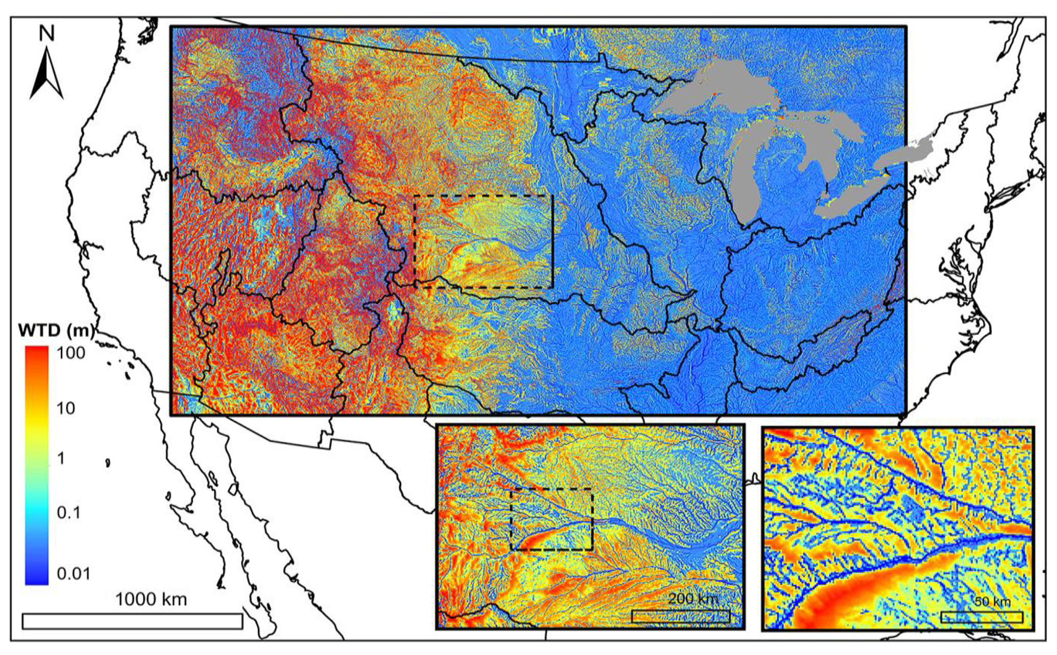
Figure 6Map of water table depth (m) over the simulation domain with two insets zooming into the North and South Platte River basin, headwaters to the Mississippi River. Colors represent depth in log scale (from 0.01 to 100 m) (reproduced from Maxwell et al., 2015). The domain uses 1 km2 grid cells and represents one of the largest and highest-resolution domains simulated by integrated models to date.
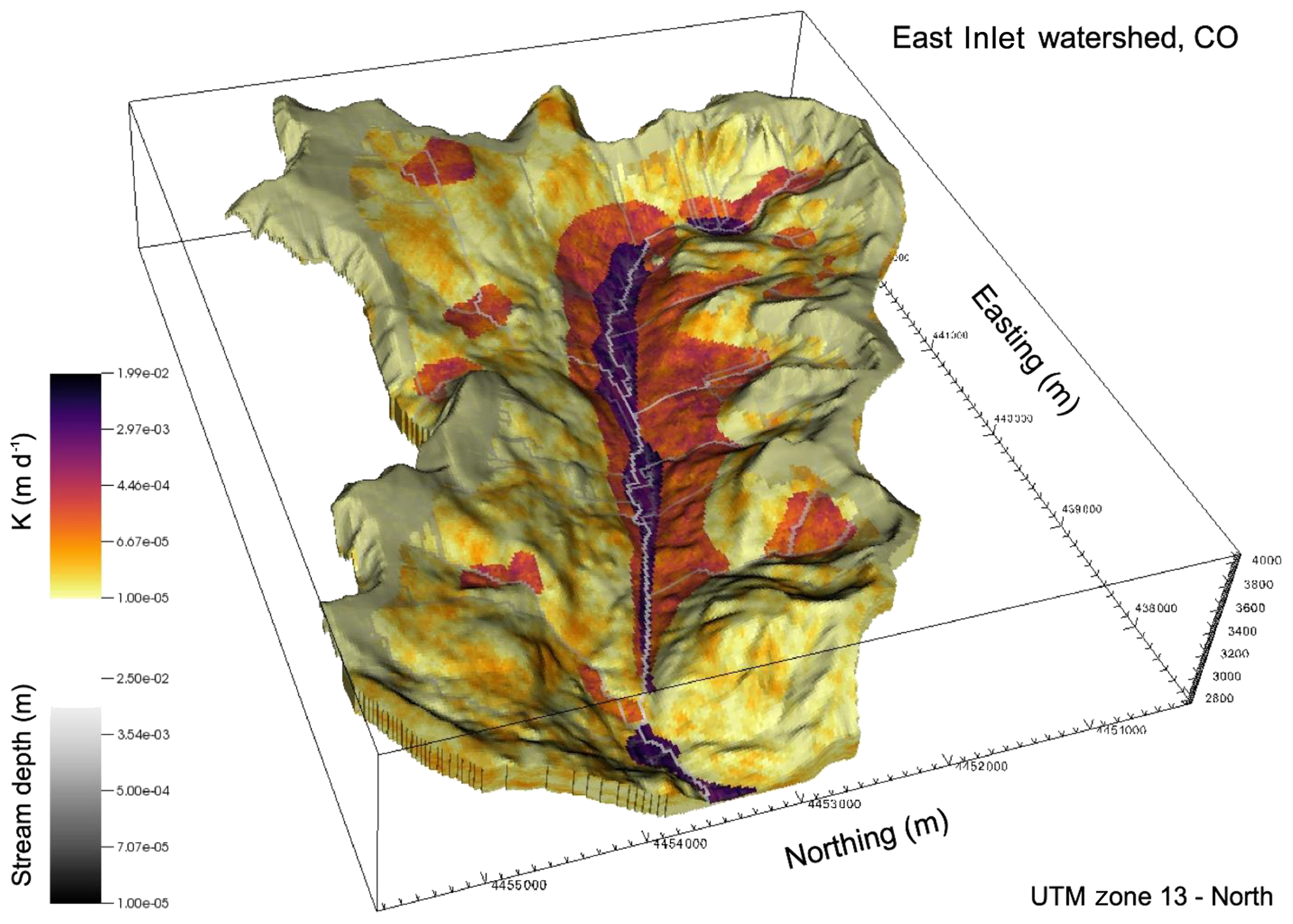
Figure 7Map of hydraulic conductivity (K) and stream depth in the East Inlet watershed in Colorado (Engdahl and Maxwell, 2015). This domain covers 30 km2 using 3.1 million lateral grid cells. The springs emanating from within the hillslopes highlight the realism afforded by integrated modeling at small scales.
ParFlow is based on efficient parallelism (high performance efficiency) and robust hydrologic capabilities. The model solvers and numerical methods used are powerful, fast, robust, and stable, which has contributed to the code's excellent parallel efficiency. As stated earlier, ParFlow is very capable of simulating flows under saturated and variably saturated conditions, i.e., surface, vadose, and groundwater flows, even in highly heterogeneous environments. For example, in simulations of surface flows (i.e., solving the kinematic wave overland flow equations), ParFlow possess the ability to accurately solve streamflow (channelized flow) by using parameterized river-routing subroutines (Maxwell and Miller, 2005; Maxwell et al., 2007, 2011). ParFlow includes coupling capabilities with a flexible coupling interface that has been utilized extensively in resolving many hydrologic problems. The interface-based and process-level coupling used by ParFlow is an example for enabling high-resolution, realistic modeling. However, based on the applications, it would be worthwhile to create one, or several, generic coupling interfaces within ParFlow to make it easier to use its surface–subsurface capabilities in other simulations. Nonetheless, ParFlow has been used in coupling studies to simulate different processes and/or systems, including simulating energy and water budgets of the surface and subsurface (Rihani et al., 2010; Mikkelson et al., 2013), surface water and groundwater flows and transport (Kollet and Maxwell, 2006; Beisman, 2007; Beisman et al., 2015; Maxwell et al., 2015), and subsurface, surface, and atmospheric mass and energy balance (Maxwell and Miller, 2005; Maxwell et al., 2011; Shrestha et al., 2014; Sulis et al., 2017). Undoubtedly, such coupled model simulations come with computational burden, and ParFlow performs well in overcoming such problems, even at high spatial scales and resolutions. This capability of ParFlow (coupling with other models) is continuously being exploited by hydrologic modelers, and new couplings are consistently being established. For example, via model coupling, the entire transpiration process could be investigated, i.e., from carbon dioxide sequestration from the atmosphere by plants, to subsurface moisture dynamics and impacts, to oxygen production by plants. Likewise, land cover change effects on mountain pine beetles may be investigated via the coupling of integrated models. But these projected research advances can only be achieved if the scientific community keeps advancing code performance by developing, revising, updating, and rigorously testing these model capabilities.
Presently, ParFlow's open-source model and open developer community is fully transparent, and this openness is a major difference between it and other models that has enabled ParFlow to continue evolving. The user community is growing daily across the globe. Code developers have made available, aside from the ParFlow working manual, an active and frequently updated blog (current blog: http://parflow.blogspot.com/, last access: 13 July 2019) and other sources including https://www.parflow.org (last access: 13 July 2019) and https://github.com/parflow (last access: 13 July 2019), where code developers and experienced users provide great information and suggestions that help fix bugs and ease the frustrations of other users. Over the years, these easily accessible resources have proven to be helpful. The code is constantly updated through the release of new versions with modifications designed to meet varying hydrologic challenges and directions for applications across different scales and fields. Each ParFlow package (version) comes with verified simulation test cases with directions that simulate different real systems and idealized cases. These serve as a great resource wherein additional code modifications have been tested in every release of the code. ParFlow has a clear, rigorous verification procedure to make sure that any changes checked in do not “break” previous developments. This ensures numerical accuracy and backwards compatibility. Moreover, the full suite of test cases is automatically rerun before any submitted change can even be considered for merging with the master branch of the code. The number of branches and/or forks cannot be controlled in any open-source (or community) code, but any contributions to the master branch are exhaustively vetted before being pushed out to users. Further, there is a software development and sustainability plan to improve the capabilities of ParFlow, such as the incorporation of new formulations of both kinematic and diffusive wave approximations and advanced parallelization support (GPUs and heterogeneous compute architectures). ParFlow works very well on different computing architectures and operating systems from “laptops to supercomputers” (single CPU, Linux clusters, highly scalable systems including IBM Blue Gene) with the same source code and input on all platforms. The code can use significant computational power and runs efficiently on supercomputing environments (e.g., Edison, Cori, JUQUEEN, and Yellowstone). Through ParFlow hydrologic modelers have available a very efficient yet still growing integrated hydrologic model to simulate and understand surface–subsurface flows.
ParFlow is an open-source, object-oriented, parallel watershed flow model developed by the community of scientists from the Environmental Protection Department at the Lawrence Livermore National Laboratory (LLNL), Colorado School of Mines, and FZ Jülich, along with supporting scientists from several other institutions. The current version of ParFlow is available at https://github.com/parflow/parflow/releases/tag/v3.6.0 (last access: 4 September 2019; Smith, 2019). The version of ParFlow described in this paper is archived on Zenodo: https://doi.org/10.5281/zenodo.3555297 (Kuffour, 2019).
Section 3 of the paper was written by CSW. BNOK and NBE wrote the other sections, and the entire paper was edited by LEC, SK, and RMM.
The authors declare that they have no conflict of interest.
We kindly acknowledge funding of the project by the U.S. Department of Energy, Office of Science (Subsurface Biogeochemical Research), award number DE-SC0019123.
This research has been supported by the U.S. Department of Energy, Office of Science (Subsurface Biogeochemical Research) (grant no. DE-SC0019123).
This paper was edited by Jeffrey Neal and reviewed by two anonymous referees.
Abu-El-Sha'r, W. Y. and Rihani, J. F.: Application of the high performance computing techniques of parflow simulator to model groundwater flow at Azraq basin, Water Resour. Manage., 21, 409–425, https://doi.org/10.1007/s11269-006-9023-5, 2007.
Ajami, H., McCabe, H. M., Evans, J. P., and Stisen, S.: Assessing the impact of model spin-up on surface water-groundwater interactions using an integrated hydrologic model, Water Resour. Res., 50, 2636–2656, https://doi.org/10.1002/2013WR014258, 2014.
Ajami, H., McCabe, M. F., and Evans, J. P.: Impacts of model initialization on an integrated surface water-groundwater model, Hydrol. Process., 29, 3790–3801, https://doi.org/10.1002/hyp.10478, 2015.
Allievi, A. and Calisal, S. M.: Application of Bubnov-Galerkin formulation to orthogonal grid generation, J. Comput. Phys., 98, 163–173, https://doi.org/10.1016/0021-9991(92)90181-W, 1992.
Amdahl, G. M.: Validity of the single processor approach to achieving large scale computing capabilities, in spring joint computer conference, Vol. 37, 256–259, 1967.
Anyah, R. O., Weaver, C. P., Miguez-Macho, G., Fan, Y., and Robock, A.: Incorporating water table dynamics in climate modeling: 3. Simulated groundwater influence on coupled land-atmosphere variability, J. Geophys. Res.-Atmos., 113, 1–15, https://doi.org/10.1029/2007JD009087, 2008.
Ashby, S. F. and Falgout, R. D.: A Parallel Multigrid Preconditioned Conjugate Gradient Algorithm for Groundwater Flow Simulations, Nucl. Sci. Eng., 124, 145–159, 1996.
Ashby, S. F., Falgout, R. D., Smith, S. G., and Tompson, A. F. B.: Modeling groundwater flow on MPPs, Proc. Scalable Parallel Libr. Conf., 17–25, https://doi.org/10.1109/SPLC.1993.365586, 1993.
Ashby, S. F., Falgout, R. D., Tompson, A., and Fogwell, T.: Numerical simulation of groundwater flow on MPPs, 17–25, 1994.
Ashby, S. F., Falgout, R. D., and Tompson, A. F. B.: A Scalable Approach to Modeling Groundwater Flow on Massively Parallel Computers, in In Next Generation Environmental Models and Computational Methods, Vol. 87, 201, 1997.
Atchley, A. L. and Maxwell, R. M.: Influences of subsurface heterogeneity and vegetation cover on soil moisture, surface temperature and evapotranspiration at hillslope scales, Hydrogeol. J., 19, 289–305, https://doi.org/10.1007/s10040-010-0690-1, 2011.
Atchley, A. L., Maxwell, R. M., and Navarre-Sitchler, A. K.: Human health risk assessment of CO2 leakage into overlying aquifers using a stochastic, geochemical reactive transport approach, Environ. Sci. Technol., 47, 5954–5962, https://doi.org/10.1021/es400316c, 2013.
Baldauf, M., Seifert, A., Forstner, J., Majewski, D., and Raschendorfer, M.: Operational Convective-Scale Numerical Weather Prediction with the COSMO Model?: Description and Sensitivities, Am. Meteorol. Soc., 3887–3905, https://doi.org/10.1175/MWR-D-10-05013.1, 2011.
Beisman, J.: Development of a parallel reactive transport model with spatially variable nitrate reduction in a floodplain aquifer, A thesis submitted to the Faculty and the Board of Trustees of the Colorado School of Mines in partial fulfillment of the requirements for the degree of Master of Science (Hydrology), 2007.
Beisman, J. J., Maxwell, R. M., Navarre-Sitchler, A. K., Steefel, C. I., and Molins, S.: ParCrunchFlow: an efficient, parallel reactive transport simulation tool for physically and chemically heterogeneous saturated subsurface environments, Comput. Geosci., 19, 403–422, https://doi.org/10.1007/s10596-015-9475-x, 2015.
Benson, D. A., Aquino, T., Bolster, D., Engdahl, N., Henri, C. V., and Fernandez-Garcia, D.: A comparison of Eulerian and Lagrangian transport and non-linear reaction algorithms, Adv. Water Resour., 99, 15–37, 2017.
Bettems, J. M., Asensio, H., Bonafe, Duniec, G., Fuhrer, O., Helmert, J., Heret, C., Kazakova, E., Lange, Machulskaya, E., Mazur, A., De Morsier, G., Rianna, G., Rozinkina, I., Vieli, B., and Vogel, G.: The COSMO Priority Project “COLOBOC”: Final Technical Report No 27, 2015.
Beven, K.: Robert E. Horton's perceptual model of infiltration processes, Hydrol. Process., 18, 3447–3460, https://doi.org/10.1002/hyp.5740, 2004.
Bhaskar, A. S., Welty, C., Maxwell, R. M., and Miller, A. J.: Untangling the effects of urban development on subsurface storage in Baltimore, Water Resour. Res., 51, 1158–1181, https://doi.org/10.1002/2014WR016039, 2015.
Briggs, W. L., Henson, V. E., and McCormick, S. F.: A Multigrid Tutorial, 72, Siam, ISBN 13978-0898714623, https://doi.org/10.1137/1.9780898719505, 2000.
Brown, P. N. and Saad, Y.: Hybrid Krylov Methods for Nonlinear Systems of Equations, SIAM J. Sci. Stat. Comput., 11, 450–481, https://doi.org/10.1137/0911026, 1990.
Burstedde, C., Fonseca, J. A., and Kollet, S.: Enhancing speed and scalability of the ParFlow simulation code, Comput. Geosci., 22, 347–361, https://doi.org/10.1007/s10596-017-9696-2, 2018.
Camporese, M., Paniconi, C., Putti, M., and Orlandini, S.: Surface-subsurface flow modeling with path-based runoff routing, boundary condition-based coupling, and assimilation of multisource observation data, Water Resour. Res., 46, W02512, https://doi.org/10.1029/2008WR007536, 2010.
Castronova, A. M., Goodall, J. L., and Ercan, M. B.: Integrated modeling within a hydrologic information system: an OpenMI based approach, Environ. Model. Softw., 39, 263–273, 2013.
Celia, M. A., Bouloutas, E. T., and Zarba, R. L.: A general mass-conservative numerical solution for the unsaturated flow equation, Water Resour. Res., 26, 1483–1496, https://doi.org/10.1029/WR026i007p01483, 1990.
Chow, F. K., Kollet, S. J., Maxwell, R. M., and Duan, Q.: Effects of Soil Moisture Heterogeneity on Boundary Layer Flow with Coupled Groundwater, Land-Surface, and Mesoscale Atmospheric Modeling, 17th Symp. Bound. Laters Turbul., https://doi.org/10.1016/j.phrs.2010.10.003, 2006.
Collier, A. M., Hindmarsh, A. C., Serban, R., and Woodward, C. S.: User Documentation for kinsol v2.8.2 (SUNDIALS v2.6.2), 1, 120, 2015.
Condon, L. E. and Maxwell, R. M.: Implementation of a linear optimization water allocation algorithm into a fully integrated physical hydrology model, Adv. Water Resour., 60, 135–147, https://doi.org/10.1016/j.advwatres.2013.07.012, 2013.
Condon, L. E. and Maxwell, R. M.: Groundwater-fed irrigation impacts spatially distributed temporal scaling behavior of the natural system: a spatio-temporal framework for understanding water management impacts, Environ. Res. Lett., 9, 034009, https://doi.org/10.1088/1748-9326/9/3/034009, 2014.
Condon, L. E. and Maxwell, R. M.: Evaluating the relationship between topography and groundwater using outputs from a continental-scale integrated hydrology model, Water Resour. Res., 51, 6602–6621, https://doi.org/10.1002/2014WR016774, 2015.
Condon, L. E., Maxwell, R. M., and Gangopadhyay, S.: The impact of subsurface conceptualization on land energy fluxes, Adv. Water Resour., 60, 188–203, https://doi.org/10.1016/J.ADVWATRES.2013.08.001, 2013.
Condon, L. E., Hering, A. S., and Maxwell, R. M.: Quantitative assessment of groundwater controls across major US river basins using a multi-model regression algorithm, Adv. Water Resour., 82, 106–123, https://doi.org/10.1016/J.ADVWATRES.2015.04.008, 2015.
Dai, Y., Zeng, X., Dickinson, R. E., Baker, I., Bonan, G. B., Bosilovich, M. G., Denning, A. S., Dirmeyer, P. A., Houser, P. R., Niu, G., and Oleson, K. W.: The Common Land Model, B. Am. Meteorol. Soc., 84, 1013–1023, https://doi.org/10.1175/BAMS-84-8-1013, 2003.
Dembo, R. S. and Eisenstat, S. C.: Inexact newton methods, in: SIAM J. Numer. Anal., Vol. 19, 400–408, 1982.
Dennis Jr., J. E. and Schnabel, R. B.: Numerical methods for unconstrained optimization and nonlinear equations, Vol. 16, Siam, 1996.
Duniec, G. and Mazur, A.: COLOBOC-MOSAIC parameterization in COSMO model v. 4.8, COSMO Newsletter, 11, 69–81, 2011.
Durbin, P.: An Approach to Local Refinement of Structured Grids An Approach to Local Refinement of Structured Grids, J. Comput. Phys., 181, 639–653, https://doi.org/10.1006/jcph.2002.7147, 2002.
Eca, L.: 2D orthogonal grid generation with boundary point distribution control, J. Comput. Phys., 125, 440–453, https://doi.org/10.1006/jcph.1996.0106, 1996.
Eisenstat, S. C. and Walker, H. F.: Choosing the Forcing Terms in an Inexact Newton Method, SIAM J. Sci. Comput., 17, 16–32, https://doi.org/10.1137/0917003, 1996.
Ek, M. B., Mitchell, K. E., Lin, Y., Rogers, E., Grunmann, P., Koren, V., Gayno, G., and Tarpley, J. D.: Implementation of Noah land surface model advances in the National Centers for Environmental Prediction operational mesoscale Eta model, J. Geophys. Res.-Atmos., 108, 8851, https://doi.org/10.1029/2002JD003296, 2003.
Engdahl, N. B. and Maxwell, R. M.: Quantifying changes in age distributions and the hydrologic balance of a high-mountain watershed from climate induced variations in recharge, J. Hydrol., 522, 152–162, https://doi.org/10.1016/j.jhydrol.2014.12.032, 2015.
Engdahl, N. B., McCallum, J. L., and Massoudieh, A.: Transient age distributions in subsurface hydrologic systems, J. Hydrol., 543, 88–100, 2016.
Falgout, R. D. and Yang, U. M.: Hypre: A Library of High Performance Preconditioners, in International Conference on Computational Science, 632–641, Springer, Berlin, 2002.
Falgout, R. D., Baldwin, C., Bosl, W., Hornung, R., Shumaker, D., Smith, S., Woodward, C. S., and Tompson, A. F. B.: Enabling computational technologies for subsurface simulations, No. UCRL-ID-133255, 97-ERD-035, WM1025000, Lawrence Livermore National Lab., CA (US), 1999.
Ferguson, I. M. and Maxwell, R. M.: Groundwater-Land Surface-Atmosphere Feedbacks: Impacts of Groundwater Pumping and Irrigation on Land-Atmosphere Interactions, Proc. xviii Int. Conf. Comput. Methods Water Resour., 722–729, 2010.
Ferguson, I. M. and Maxwell, R. M.: Hydrologic and land-energy feedbacks of agricultural water management practices, Environ. Res. Lett., 6, 014006, https://doi.org/10.1088/1748-9326/6/1/014006, 2011.
Ferguson, I. M. and Maxwell, R. M.: Human impacts on terrestrial hydrology: climate change versus pumping and irrigation, Environ. Res. Lett., 7, 044022, https://doi.org/10.1088/1748-9326/7/4/044022, 2012.
Ferguson, I. M., Jefferson, J. L., Maxwell, R. M., and Kollet, S. J.: Effects of root water uptake formulation on simulated water and energy budgets at local and basin scales, Environ. Earth Sci., 75, 316, https://doi.org/10.1007/s12665-015-5041-z, 2016.
Frei, S., Fleckenstein, J. H., Kollet, S. J., and Maxwell, R. M.: Patterns and dynamics of river-aquifer exchange with variably-saturated flow using a fully-coupled model, J. Hydrol., 375, 383–393, https://doi.org/10.1016/j.jhydrol.2009.06.038, 2009.
Gasper, F., Goergen, K., Shrestha, P., Sulis, M., Rihani, J., Geimer, M., and Kollet, S.: Implementation and scaling of the fully coupled Terrestrial Systems Modeling Platform (TerrSysMP v1.0) in a massively parallel supercomputing environment – a case study on JUQUEEN (IBM Blue Gene/Q), Geosci. Model Dev., 7, 2531–2543, https://doi.org/10.5194/gmd-7-2531-2014, 2014.
Gebler, S., Kollet, S., Qu, W., and Vereecken, H.: High resolution modelling of soil moisture patterns with ParFlow-CLM?: Comparison with sensor network data, in: EGU General Assembly Conference Abstracts, 17, 2015.
Gilbert, J. M. and Maxwell, R. M.: Examining regional groundwater–surface water dynamics using an integrated hydrologic model of the San Joaquin River basin, Hydrol. Earth Syst. Sci., 21, 923–947, https://doi.org/10.5194/hess-21-923-2017, 2017.
Gustafson, J. L.: Reevaluating amdahl's law, Communications of the ACM, 31, 532–533, 1988.
Haussling, H. and Coleman, R.: A method for generation of orthogonal and nearly orthogonal boundary-fitted coordinate systems, J. Comput. Phys., 43, 373–381, https://doi.org/10.1016/0021-9991(81)90129-7, 1981.
Hindmarsh, A. C., Brown, P. N., Grant, K. E., Lee, S. L., Serban, R., Shumaker, D. E., and Woodward, C. S.: SUNDIALS: Suite of nonlinear and differential/algebraic equation solvers, ACM Trans. Math. Softw., 31, 363–396, https://doi.org/10.1145/1089014.1089020, 2005.
Jefferson, J. L. and Maxwell, R. M.: Evaluation of simple to complex parameterizations of bare ground evaporation, J. Adv. Model. Earth Syst., 7, 1075–1092, https://doi.org/10.1002/2014MS000398, 2015.
Jefferson, J. L., Gilbert, J. M., Constantine, P. G., and Maxwell, R.M.: Active subspaces for sensitivity analysis and dimension reduction of an integrated hydrologic model, Comput. Geosci., 83, 127–138, https://doi.org/10.1016/j.cageo.2015.07.001, 2015.
Jefferson, J. L., Maxwell,R. M., and Constantine, P. G.: Exploring the Sensitivity of Photosynthesis and Stomatal Resistance Parameters in a Land Surface Model, J. Hydrometeorol., 18, 897–915, https://doi.org/10.1175/JHM-D-16-0053.1, 2017.
Jiang, X., Niu, G. Y., and Yang, Z. L.: Impacts of vegetation and groundwater dynamics on warm season precipitation over the Central United States, J. Geophys. Res.-Atmos., 114, 1–15, https://doi.org/10.1029/2008JD010756, 2009.
Jones, J. E. and Woodward, C. S.: Preconditioning Newton- Krylov Methods for Variably Saturated Flow, in 13th International Conference on Computational Methods in Water Resources, Calgary, Alberta, Canada, 2000.
Jones, J. E. and Woodward, C. S.: Newton-Krylov-multigrid solvers for large-scale, highly heterogeneous, variably saturated flow problems, Adv. Water Resour., 24, 763–774, https://doi.org/10.1016/S0309-1708(00)00075-0, 2001.
Keune, J., Gasper, F., Goergen, K., Hense, A., Shrestha, P., Sulis, M., and Kollet, S.: Studying the influence of groundwater representations on land surface-atmosphere feedbacks during the European heat wave in 2003, J. Geophys. Res., 121, 13301–13325, https://doi.org/10.1002/2016JD025426, 2016.
Khorsandi, E., Kollet, S., Venema, V., and Simmer, C.: Investigating the effect of bottom boundary condition placement on ground heat storage in climate time scale simulations using ParflowE, Geophys. Res., 16, EGU2014-931, https://doi.org/10.1029/2006GL028546, 2014.
Kirkner, D. J. and Reeves, H.: Multicomponent Mass Transport With Homogeneous and Heterogeneous Chemical Reactions' Effect of the Chemistry on the Choice of Numerical Algorithm 1. Theory, Water Resour. Res., 24, 1719–1729, 1988.
Koch, J., Cornelissen, T., Fang, Z., Bogena, H., Diekkrüger, B., Kollet, S., and Stisen, S.: Inter-comparison of three distributed hydrological models with respect to seasonal variability of soil moisture patterns at a small forested catchment, J. Hydrol., 533, 234–249, https://doi.org/10.1016/j.jhydrol.2015.12.002, 2016.
Kollet, S., Sulis, M., Maxwell, R. M., Paniconi, C., Putti, M., Bertoldi, G., Coon, E. T., Cordano, E., Endrizzi S., Kikinzon, E., Mouche, E., Mugler, C., Park, Y., Refsgaard, J. C., Stisen, S., and Sudicky, E.: The integrated hydrologic model intercomparison project, IH‐MIP2: A second set of benchmark results to diagnose integrated hydrology and feedbacks, Water Resour. Res., 53, 867–890, 2017.
Kollet, S. J.: Influence of soil heterogeneity on evapotranspiration under shallow water table conditions: transient, stochastic simulations, Environ. Res. Lett., 4, 035007, https://doi.org/10.1088/1748-9326/4/3/035007, 2009.
Kollet, S. J.: Technical note: Inference in hydrology from entropy balance considerations, Hydrol. Earth Syst. Sci., 20, 2801–2809, https://doi.org/10.5194/hess-20-2801-2016, 2016.
Kollet, S. J. and Maxwell, R. M.: Integrated surface-groundwater flow modeling: A free-surface overland flow boundary condition in a parallel groundwater flow model, Adv. Water Resour., 29, 945–958, https://doi.org/10.1016/j.advwatres.2005.08.006, 2006.
Kollet, S. J. and Maxwell, R. M.: Capturing the influence of groundwater dynamics on land surface processes using an integrated, distributed watershed model, Water Resour. Res., 44, 1–18, https://doi.org/10.1029/2007WR006004, 2008a.
Kollet, S. J. and Maxwell, R. M.: Demonstrating fractal scaling of baseflow residence time distributions using a fully-coupled groundwater and land surface model, Geophys. Res. Lett., 35, 1–6, https://doi.org/10.1029/2008GL033215, 2008b.
Kollet, S. J., Cvijanovic, I., Schüttemeyer, D., Maxwell, R. M., Moene, A. F., and Bayer, P.: The Influence of Rain Sensible Heat and Subsurface Energy Transport on the Energy Balance at the Land Surface, Vadose Zone J., 8, 846, https://doi.org/10.2136/vzj2009.0005, 2009.
Kollet, S. J., Maxwell, R. M., Woodward, C. S., Smith, S., Vanderborght, J., Vereecken, H., and Simmer, C.: Proof of concept of regional scale hydrologic simulations at hydrologic resolution utilizing massively parallel computer resources, Water Resour. Res., 46, 1–7, https://doi.org/10.1029/2009WR008730, 2010.
Kuffour, B. N. O.: Parflow-350/parflow: ParFlow Version 3.5.0, Zenodo, https://doi.org/10.5281/zenodo.3555297, 2019.
Kumar, M., Duffy, C. J., and Salvage, K. M.: A second-order accurate, finite volume–based, integrated hydrologic modeling (FIHM) framework for simulation of surface and subsurface flow, Vadose Zone J., 8, 873, https://doi.org/10.2136/vzj2009.0014, 2009.
LaBolle, E. M., Ahmed, A. A., and Fogg, G. E.: Review of the Integrated Groundwater and Surface-Water Model (IGSM), Ground Water, 41, 238–246, https://doi.org/10.1111/j.1745-6584.2003.tb02587.x, 2003.
Levis, S. and Jaeger, E. B.: COSMO-CLM2?: a new version of the COSMO- CLM model coupled to the Community Land Model coupled to the Community Land Model, Clim. Dynam., 37, 1889–1907, https://doi.org/10.1007/s00382-011-1019-z, 2011.
Li, L., Steefel, C. I., Kowalsky, M. B., Englert, A., and Hubbard, S. S.: Effects of physical and geochemical heterogeneities on mineral transformation and biomass accumulation during uranium bioremediation at Rifle, Colorado, J. Contam. Hydrol., 11, 45–63, 2010.
Li, L., Steefel, C. I., and Yang, L.: Scale dependence of mineral dissolution rates within single pores and fractures, Geochim. Cosmochim. Acta, 72, 360–377, https://doi.org/10.1016/j.gca.2007.10.027, 2007.
Markstrom, S. L., Niswonger, R. G., Regan, R. S., Prudic, D. E., and Barlow, P. M.: GSFLOW – Coupled Ground-Water and Surface-Water Flow Model Based on the Integration of the Precipitation-Runoff Modeling System (PRMS) and the Modular Ground-Water Flow Model (MODFLOW-2005), U.S. Geol. Surv., (Techniques and Methods 6-D1), 240, 2008.
Maxwell, R. M. and Miller, N. L.: Development of a Coupled Land Surface and Groundwater Model, J. Hydrometeorol., 6, 233–247, https://doi.org/10.1175/JHM422.1, 2005.
Maxwell, R. M.: Infiltration in Arid Environments: Spatial Patterns between Subsurface Heterogeneity and Water-Energy Balances, Vadose Zone J., 9, 970, https://doi.org/10.2136/vzj2010.0014, 2010.
Maxwell, R. M.: A terrain-following grid transform and preconditioner for parallel, large-scale, integrated hydrologic modeling, Adv. Water Resour., 53, 109–117, https://doi.org/10.1016/j.advwatres.2012.10.001, 2013.
Maxwell, R. M., Welty, C., and Tompson, A. F. B.: Streamline-based simulation of virus transport resulting from long term artificial recharge in a heterogeneous aquifer, Adv. Water Resour., 26, 1075–1096, https://doi.org/10.1016/S0309-1708(03)00074-5, 2003.
Maxwell, R. M., Chow, F. K., and Kollet, S. J.: The groundwater–land-surface–atmosphere connection: Soil moisture effects on the atmospheric boundary layer in fully-coupled simulations, Adv. Water Resour., 30, 2447–2466, https://doi.org/10.1016/j.advwatres.2007.05.018, 2007.
Maxwell, R. M., Lundquist, J. K., Mirocha, J. D., Smith, S. G., Woodward, C. S., and Tompson, A. F. B.: Development of a Coupled Groundwater–Atmosphere Model, Mon. Weather Rev., 139, 96–116, https://doi.org/10.1175/2010MWR3392.1, 2011.
Maxwell, R. M., Putti, M., Meyerhoff, S., Delfs, J., Ferguson, I. M., Ivanov, V., Kim, J., Kolditz, O., Kollet, S. J., Kumar, M., Lopez, S., Niu, J., Paniconi, C., Park, Y., Phanikumar, M. S., Shen, C., Sudicky, A., and Sulis, M.: Surface-subsurface model intercomparison: A first set of benchmark results to diagnose integrated hydrology and feedbacks, Water Resour. Res., 50, 1531–1549, https://doi.org/10.1002/2013WR013725, 2014.
Maxwell, R. M., Condon, L. E., and Kollet, S. J.: A high-resolution simulation of groundwater and surface water over most of the continental US with the integrated hydrologic model ParFlow v3, Geosci. Model Dev., 8, 923–937, https://doi.org/10.5194/gmd-8-923-2015, 2015.
Maxwell, R. M., Kollet, S. J., Smith, S. G., Woodward, C. S., Falgout, R. D., Ferguson, I. M., Engdahl, N. B., Condon, L. E., Hector, B., Lopez, S., Gilbert, J., Bearup, L., Jefferson, J., Collins, C., De Graaf, I., Pribulick, C., Baldwin, C., Bosl, W. J., Hornung, R., and Ashby, S.: ParFlow User's Manual, Integrated GroundWater Modeling Center Report GWMI, 167 p., 2016.
Meehl, G. A., Covey, C., McAvaney, B., Latif, M., and Stouffer, R. J.: Overview of the coupled model intercomparison project, B. Am. Meteorol. Soc., 86, 89–93, https://doi.org/10.1175/BAMS-86-1-89, 2005.
Meyerhoff, S. B. and Maxwell, R. M.: Using an integrated surface-subsurface model to simulate runoff from heterogeneous hillslopes, in xviii International Conference on Water Resources, CIMNE, Barcelona, 2010.
Michalakes, J., Dudhia, J., Gill, D., Klemp, J., and Skamarock, W.: Design of a next-generation regional weather research and forecast model, Towar. Teracomputing, 1999.
Michalakes, J., Chen, S., Dudhia, J., Hart, L., Klemp, J., Middlecoff, J., and Skamarock, W.: Development of a next-generation regional weather research and forecast model, Towar. Teracomputing, 2001.
Mikkelson, K. M., Maxwell, R. M., Ferguson, I., Stednick, J. D., Mccray, J. E., and Sharp, J. O.: Mountain pine beetle infestation impacts: Modeling water and energy budgets at the hill-slope scale, Ecohydrology, 6, 64–72, https://doi.org/10.1002/eco.278, 2013.
Mironov, D., Heise, E., Kourzeneva, E., and Ritter, B.: Implementation of the lake parameterisation scheme FLake into the numerical weather prediction model COSMO, Boreal Environ. Res., 6095, 218–230, 2010.
Mobley, C. D. and Stewart, R. S.: On the numerical generation of boundary-fitted orthogonal curvilinear coordinate systems, J. Comput. Phys., 34, 124–135, https://doi.org/10.1016/0021-9991(80)90117-5, 1980.
Molders, N. and Ruhaak, W.: On the impact of explicitly predicted runoff on the simulated atmospheric response to small-scale land-use changes – an integrated modeling approach, Atmos. Res., 63, 3–38, 2002.
Navarre-Sitchler, A., Steefel, C. I., Sak, P. B., and Brantley, S. L.: A reactive-transport model for weathering rind formation on basalt, Geochim. Cosmochim. Acta, 75, 7644–7667, https://doi.org/10.1016/j.gca.2011.09.033, 2011.
Oleson, K. W., Niu, G. Y., Yang, Z. L., Lawrence, D. M., Thornton, P. E., Lawrence, P. J., Stockli, R., Dickinson, R. E., Bonan, G. B., Levis, S., Dai, A., and Qian, T.: Improvements to the Community Land Model and their impact on the hydrological cycle, J. Geophys. Res.-Biogeosci., 113, G01021, https://doi.org/10.1029/2007JG000563, 2008.
Osei-Kuffuor, D., Maxwell, R. M., and Woodward, C. S.: Improved numerical solvers for implicit coupling of subsurface and overland flow, Adv. Water Resour., 74, 185–195, https://doi.org/10.1016/j.advwatres.2014.09.006, 2014.
Panday, S. and Huyakorn, P. S.: A fully coupled physically-based spatially-distributed model for evaluating surface/subsurface flow, Adv. Water Resour., 27, 361–382, https://doi.org/10.1016/j.advwatres.2004.02.016, 2004.
Rahman, M., Sulis, M., and Kollet, S. J.: Evaluating the dual-boundary forcing concept in subsurface-land surface interactions of the hydrological cycle, Hydrol. Process., 30, 1563–1573, https://doi.org/10.1002/hyp.10702, 2016.
Ren, D. and Xue, M.: A revised force–restore model for land surface modeling, Am. Meteorol. Soc., 43, 1768–1782, 2004.
Reyes, B., Maxwell, R. M., and Hogue, T. S.: Impact of lateral flow and spatial scaling on the simulation of semi-arid urban land surfaces in an integrated hydrologic and land surface model, Hydrol. Process., 30, 1192–1207, https://doi.org/10.1002/hyp.10683, 2016.
Richards, L. A.: Capillary conduction of liquids through porous mediums, J. Appl. Phys., 1, 318–333, https://doi.org/10.1063/1.1745010, 1931.
Rihani, J. F., Maxwell, M. R., and Chow, F. K.: Coupling groundwater and land surface processes: Idealized simulations to identify effects of terrain and subsurface heterogeneity on land surface energy fluxes, Water Resour. Res., 46, 1–14, https://doi.org/10.1029/2010WR009111, 2010.
Rihani, J. F., Chow, F. K., Fotini K., and Maxwell, R. M.: Isolating effects of terrain and soil moisture heterogeneity on the atmospheric boundary layer: Idealized simulations to diagnose land-atmosphere feedbacks, J. Adv. Model. Earth Syst., 6, 513–526, https://doi.org/10.1002/2014MS000371.Received, 2015.
Ryskin, G. and Leal, L.: Orthogonal mapping, J. Comput. Phys., 50, 71–100, https://doi.org/10.1016/0021-9991(83)90042-6, 1983.
Saad, Y. and Schultz, M. H.: GMRES: A Generalized Minimal Residual Algorithm for Solving Nonsymmetric Linear Systems, SIAM J. Sci. Stat. Comput., 7, 856–869, https://doi.org/10.1137/0907058, 1986.
Seck, A., Welty, C., and Maxwell, R. M.: Spin-up behavior and effects of initial conditions for an integrated hydrologic model, Water Resour. Res., 51, 2188–2210, https://doi.org/10.1002/2014WR016371, 2015.
Seuffert, G., Gross, P., Simmer, A. C., and Wood, E. F.: The Influence of Hydrologic Modeling on the Predicted Local Weather: Two-Way Coupling of a Mesoscale Weather Prediction Model and a Land Surface Hydrologic Model, J. Hydrometeorol., 3, 505–523, 2002.
Shen, C. and Phanikumar, M. S.: A process-based, distributed hydrologic model based on a large-scale method for surface-subsurface coupling, Adv. Water Resour., 33, 1524–1541, https://doi.org/10.1016/j.advwatres.2010.09.002, 2010.
Shi, Y., Davis, K. J., Zhang, F., and Duffy, C. J.: Evaluation of the Parameter Sensitivities of a Coupled Land Surface Hydrologic Model at a Critical Zone Observatory, J. Hydrometeorol., 15, 279–299, https://doi.org/10.1175/JHM-D-12-0177.1, 2014.
Shrestha, P., Sulis, M., Masbou, M., Kollet, S., and Simmer, C.: A.: Scale-Consistent Terrestrial Systems Modeling Platform Based on COSMO, CLM, and ParFlow, Mon. Weather Rev., 142, 3466–3483, https://doi.org/10.1175/MWR-D-14-00029.1, 2014.
Shrestha, P., Sulis, M., Simmer, C., and Kollet, S.: Impacts of grid resolution on surface energy fluxes simulated with an integrated surface-groundwater flow model, Hydrol. Earth Syst. Sci., 19, 4317–4326, https://doi.org/10.5194/hess-19-4317-2015, 2015.
Simmer, C., Thiele-Eich, I., Masbou, M., Amelung, W., Bogena, H., Crewell, S., Diekkruger, B., Ewert, F., Franssen, H. H., Huisman, J. A., Kemna, A., Klitzsch, N., Kollet, S., Langensiepen, M., Lohnert, U., Mostaquimur Rhaman, A. S. M., Rascher, U., Schneider, K., Schween, J., Shao, Y., Shrestha, P., Stiebler, M., Sulis, M., Vanderborght, J., Vereecken, H., Kruk, J. V. D., Waldhoff, G., and Zerenner, T. : Monitoring and modeling the terrestrial system from pores to catchments: The transregional collaborative research center on patterns in the soil-vegetation-atmosphere system, B. Am. Meteorol. Soc., 96, 1765–1787, https://doi.org/10.1175/BAMS-D-13-00134.1, 2015.
Skamarock, W. C. and Klemp, J. B.: A Time-Split Nonhydrostatic Atmospheric Model for Weather Research and Forecasting Applications, J. Comput. Phys, 7, 1–43, 2007.
Skamarock, W. C., Klemp, J. B., Dudhia, J., Gill, D. O., Barker, D. M., Wang, W., and Powers, J. G.: A description of the advanced research WRF Version 2, NCAR Tech, p. 88, Note NCAR/TN-4681STR, 2005.
Smith, S.: ParFlow Version 3.6.0, available at: https://github.com/parflow/parflow/releases/tag/v3.6.0, last access: 4 September 2019.
Smith, S. G., Ashby, S. F., Falgout, R. D., and Tompsom, A. F. B.: The parallel performance of a groundwater flow code on the CRAY T3D, in: Proceedings of the Seventh SIAM Conference on Parallel Processing for Scientific Computing, 131, 1995.
Srivastava, V., Graham, W., Muñoz-Carpena, R., and Maxwell, R. M.: Insights on geologic and vegetative controls over hydrologic behavior of a large complex basin – Global Sensitivity Analysis of an integrated parallel hydrologic model, J. Hydrol., 519, 2238–2257, 2014.
Steefel, C. I.: CrunchFlow Software for Modeling Multicomponent Reactive Flow and Transport User's Manual, 2009.
Steefel, C. I. and Lasaga, A. C.: A coupled model for transport of multiple chemical species and kinetic precipitation/dissolution reactions with application to reactive flow in single phase hydrothermal systems, Am. J. Sci., 294, 529–592, https://doi.org/10.2475/ajs.294.5.529, 1994.
Steefel, C. I. and Van Cappellen, P.: A new kinetic approach to modeling water-rock interaction: The role of nucleation, precursors, and Ostwald ripening, Geochim. Cosmochim. Acta, 54, 2657–2677, https://doi.org/10.1016/0016-7037(90)90003-4, 1990.
Steefel, C. I. and Yabusaki, S. B.: OS3D/GIMRT software for modeling multicomponent-multidimensional reactive transport, Richland, WA, 1996.
Steiner, A. L., Pal, J. S., Giorgi, F., Dickinson, R. E., and Chameides, W. L.: The coupling of the Common Land Model (CLM0) to a regional climate model (RegCM), Theor. Appl. Climatol., 82, 225–243, https://doi.org/10.1007/s00704-005-0132-5, 2005.
Steiner, A. L., Pal, J. S., Rauscher, S. A., Bell, J. L., Diffenbaugh, N. S., Boone, A., Sloan, L. C., and Giorgi, F.: Land surface coupling in regional climate simulations of the West African monsoon, Clim. Dynam., 33, 869–892, https://doi.org/10.1007/s00382-009-0543-6, 2009.
Sudicky, E. A., Jones, J. P., Park, Y. J., Brookfield, A. E., and Colautti, D.: Simulating complex flow and transport dynamics in an integrated surface-subsurface modeling framework, Geosci. J., 12, 107–122, https://doi.org/10.1007/s12303-008-0013-x, 2008.
Sulis, M., Meyerhoff, S. B., Paniconi, C., Maxwell, R. M., Putti, M., and Kollet, S. J.: A comparison of two physics-based numerical models for simulating surface water-groundwater interactions, Adv. Water Resour., 33, 456–467, https://doi.org/10.1016/j.advwatres.2010.01.010, 2010.
Sulis, M., Williams, J. L., Shrestha, P., Diederich, M., Simmer, C., Kollet, S. J., and. Maxwell, R. M.: Coupling Groundwater, Vegetation, and Atmospheric Processes: A Comparison of Two Integrated Models, J. Hydrometeorol., 18, 1489–1511, https://doi.org/10.1175/JHM-D-16-0159.1, 2017.
Therrien, R. and Sudicky, E.: Three-dimensional analysis of variably-saturated flow and solute transport in discretely- fractured porous media, J. Contam. Hydrol., 23, 1–44, https://doi.org/10.1016/0169-7722(95)00088-7, 1996.
Tompson, A. F. B., Ashby, S. F., and Falgout, R. D.: Use of high performance computing to examine the effectiveness of aquifer remediation, (No. UCRL-JC–115374), Lawrence Livermore National Lab, 1994.
Tompson, A. F. B., Falgout, R. D., Smith, S. G., Bosl, W. J., and Ashby, S. F.: Analysis of subsurface contaminant migration and remediation using high performance computing, Adv. Water Resour., 22, 203–221, https://doi.org/10.1016/S0309-1708(98)00013-X, 1998.
Tompson, A. F. B., Carle, S. F., Rosenberg, N. D., and Maxwell, R. M.: Analysis of groundwater migration from artificial recharge in a large urban aquifer: A simulation perspective, Water Resour. Res., 35, 2981–2998, https://doi.org/10.1029/1999WR900175, 1999.
Valcke, S.: The OASIS3 coupler: a European climate modelling community software, Geosci. Model Dev., 6, 373–388, https://doi.org/10.5194/gmd-6-373-2013, 2013.
Valcke, S., Balaji, V., Bentley, P., Guilyardi, E., Lawrence, B., and Pascoe, C.: Developing a Common Information Model for climate models and data, Geophys. Res. Abstr., 11, 10592, 2009.
Valcke, S., Balaji, V., Craig, A., DeLuca, C., Dunlap, R., Ford, R. W., Jacob, R., Larson, J., O'Kuinghttons, R., Riley, G. D., and Vertenstein, M.: Coupling technologies for Earth System Modelling, Geosci. Model Dev., 5, 1589–1596, https://doi.org/10.5194/gmd-5-1589-2012, 2012.
VanderKwaak, J. E.: Numerical simulation of flow and chemical transport in integrated surface-subsurface hydrologic systems, A thesis presented to the University of Waterloo in fulfillment of the thesis requirement for the degree of Doctor of Philosophy Earth Sciences Waterloo, Ontario, Canada, 1999.
Van Genuchten, M. T.: A Closed-form Equation for Predicting the Hydraulic Conductivity of Unsaturated Soils, Soil Sci. Soc. Am. J., 44, 892–898, https://doi.org/10.2136/sssaj1980.03615995004400050002x, 1980.
Visbal, M. and Knight, D.: Generation of orthogonal and nearly orthogonal coordinates with gridcontrol near boundaries, AIAA J., 20, 305–306, https://doi.org/10.2514/3.7915, 1982.
Vogel, B., Vogel, H., Bäumer, D., Bangert, M., Lundgren, K., Rinke, R., and Stanelle, T.: The comprehensive model system COSMO-ART – Radiative impact of aerosol on the state of the atmosphere on the regional scale, Atmos. Chem. Phys., 9, 8661–8680, https://doi.org/10.5194/acp-9-8661-2009, 2009.
Wagner, S., Fersch, B., Yuan, Y.,Yu, Z., and Kunstmann, H.: Fully coupled atmospheric-hydrological modeling at regional and long-term scales: Development, application, and analysis of WRF-HMS, Water Resour. Res., 52, 3187–3211, https://doi.org/10.1002/2015WR018185, 2016.
Weill, S., Mouche, E., and Patin, J.: A generalized Richards equation for surface/subsurface flow modelling, J. Hydrol., 366, 9–20, https://doi.org/10.1016/j.jhydrol.2008.12.007, 2009.
Weill, S., Mazzia, A., Putti, M., and Paniconi, C.: Coupling water flow and solute transport into a physically-based surface-subsurface hydrological model, Adv. Water Resour., 34, 128–136, https://doi.org/10.1016/j.advwatres.2010.10.001, 2011.
Williams, J. L. and Maxwell, R. M.: Propagating Subsurface Uncertainty to the Atmosphere Using Fully Coupled Stochastic Simulations, J. Hydrometeorol., 12, 690–701, https://doi.org/10.1175/2011JHM1363.1, 2011.
Williams, J. L., Maxwell, R. M., and Monache, L. D.: Development and verification of a new wind speed forecasting system using an ensemble Kalman filter data assimilation technique in a fully coupled hydrologic and atmospheric model, J. Adv. Model. Earth Syst., 5, 785–800, https://doi.org/10.1002/jame.20051, 2013.
Wood, B. D.: The role of scaling laws in upscaling, Adv. Water Resour., 32, 723–736, https://doi.org/10.1016/j.advwatres.2008.08.015, 2009.
Woodward, S. C.: A Newton-Krylov-multigrid solver for variably saturated flow problems, Proceedings on the Twelfth International Conference on Computational Methods in Water Resources, in Computational Mechanics Publications, vol. 2, 609–616, 1998.
Xu, L., Raman, S., and Madala, R. V.: A review of non-hydrostatic numerical models for the atmosphere, Math. Subj. Classif, 1991.
Xue, M., Droegemeier, K. K., and Wong, V.: The Advanced Regional Prediction System (ARPS) – A multi-scale nonhydrostatic atmospheric simulation and prediction tool. Part II: Model dynamics and verification, Meteorol. Atmos. Phys., 75, 161–193, https://doi.org/10.1007/s007030170027, 2000.
Zhufeng, F., Bogena, H., Kollet, S., and Koch, J. H. V.: Spatio-temporal validation of long-term 3D hydrological simulations of a forested catchment using empirical orthogonal functions and wavelet coherence analysis, Hydrology, 529, 1754–1767, 2015.