the Creative Commons Attribution 4.0 License.
the Creative Commons Attribution 4.0 License.
 | 27 Jan 2020
SEAMUS (v1.20): a Δ14C-enabled, single-specimen sediment accumulation simulator
Bryan C. Lougheed
The systematic bioturbation of single particles (such as foraminifera) within deep-sea sediment archives leads to the apparent smoothing of any temporal signal as recorded by the downcore, discrete-depth mean signal. This smoothing is the result of the systematic mixing of particles from a wide range of depositional ages into the same discrete-depth interval. Previous sediment models that simulate bioturbation have specifically produced an output in the form of a downcore, discrete-depth mean signal. However, palaeoceanographers analysing the distribution of single foraminifera specimens from sediment core intervals would be assisted by a model that specifically evaluates the effect of bioturbation upon single specimens. Taking advantage of advances in computer memory, the single-specimen SEdiment AccuMUlation Simulator (SEAMUS) was created for MATLAB and Octave, allowing for the simulation of large arrays of single specimens. This model allows researchers to analyse the post-bioturbation age heterogeneity of single specimens contained within discrete-depth sediment core intervals and how this heterogeneity is influenced by changes in sediment accumulation rate (SAR), bioturbation depth (BD) and species abundance. The simulation also assigns a realistic 14C activity to each specimen, by considering the dynamic Δ14C history of the Earth and temporal changes in reservoir age. This approach allows for the quantification of possible significant artefacts arising when 14C-dating multi-specimen samples with heterogeneous 14C activity. Users may also assign additional desired carrier signals to single specimens (stable isotopes, trace elements, temperature, etc.) and consider a second species with an independent abundance. Finally, the model can simulate a virtual palaeoceanographer by randomly picking whole specimens (whereby the user can set the percentage of older, “broken” specimens) of a prescribed sample size from discrete depths, after which virtual laboratory 14C dating and 14C calibration is carried out within the model. The SEAMUS bioturbation model can ultimately be combined with other models (proxy and ecological models) to produce a full climate-to-sediment model workflow, thus shedding light on the total uncertainty involved in palaeoclimate reconstructions based on sediment archives.


Deep-sea sediment archives provide valuable insight into past changes in ocean circulation and global climate. The most often studied carrier vessels of the climate signal are the calcite tests of foraminifera. The tests of these organisms incorporate isotopes and trace elements of the ambient water at the time of calcification before sinking to the seafloor sediment archive after death. Each discrete-depth interval of a sediment core (typically 1 cm core slices) retrieved from the sea floor can contain many thousands of specimens. Owing to technical constraints, researchers have typically had to combine many tens or hundreds of single tests into a single sample for successful analysis using mass spectrometry. Furthermore, post-depositional sediment mixing (e.g. bioturbation; Berger and Heath, 1968) of deep-sea sediment means that foraminifera specimens of vastly differing ages can be mixed into the same discrete-depth interval. The main consequence of this mixing is that a downcore, discrete-depth multi-specimen reconstruction of a specific climate proxy will appear to be strongly smoothed out (on the order of multiple centuries or millennia) when compared to the original temporal signal (Pisias, 1983; Schiffelbein, 1984; Bard et al., 1987). Moreover, machine analysis of multi-specimen samples will only report the mean value and machine error, thus hiding the true distribution of values within the sample. Advances in mass spectrometry eventually allowed the analysis of single specimens (Killingley et al., 1981) and, since single specimens capture a single year or season of the climate signal, researchers can in principle study the full distribution of isotope or trace element values obtained within various discrete depths of sediment cores, thereby making inferences regarding variability in climate, habitat or specimen morphology for various specific time periods during the Earth's history (Spero and Williams, 1990; Tang and Stott, 1993; Billups and Spero, 1996; Ganssen et al., 2011; Wit et al., 2013; Ford et al., 2015; Metcalfe et al., 2015; Ford and Ravelo, 2019; Metcalfe et al., 2019b). However, the accuracy with which the aforementioned studies can quantify time-specific variation for a particular climate period, habitat or morphological variable is strongly dependent upon the constraint of the age range of the specimens contained within a given discrete-depth interval. The aforementioned studies still rely upon the age–depth method to assign an age range to all specimens contained within a discrete-depth interval, and previous models of single-specimen analysis in sediment cores do not include bioturbation (Thirumalai et al., 2013; Fraass and Lowery, 2017). Such an approach can be problematic if, to give but one example, an assumed Holocene-age 1 cm slice of sediment core were to also contain a significant number of Late Glacial specimens, which could lead to a spurious interpretation of Holocene climate variability. Ultimately, this problem can be circumvented through the application of paired analysis of both radiocarbon (14C) and stable isotopes on single specimens (Lougheed et al., 2018), but the current mass requirements of 14C accelerated mass spectrometry (AMS) necessitates very large specimens (>100 µg), whereas most planktonic foraminifera used in palaeoceanography are an order of magnitude smaller. Until such time that single-specimen 14C methods become systematically applicable to planktonic specimens, and for periods older than the analytical limit of 14C dating (>50 ka), a sediment accumulation model specifically designed for the analysis of single specimens can help shed light on the age (and proxy) value distributions of planktonic foraminifera contained within discrete depths.
Quantifying the distribution of specimen ages within discrete-depth sediment intervals is also important for 14C dating applied to multi-specimen samples, which can be expected to have heterogeneous radiocarbon (14C) activity. In addition to bioturbation, this 14C heterogeneity is also influenced by the Earth's dynamic Δ14C history, temporal changes in species abundance, sediment accumulation rate (SAR) and local 14C reservoir age. The resulting temporal changes in sample 14C heterogeneity have the potential to induce downcore age–depth artefacts when 14C analysis and 14C calibration are applied to multi-specimen samples. The ability to make a quantitative estimate of downcore changes in the 14C heterogeneity and its effect upon 14C dating would help to improve 14C-based chronologies.
Here, we present the Δ14C-enabled single-specimen SEdiment AccuMUlation Simulator (SEAMUS), which can help researchers quantify the affect of bioturbation upon single foraminifera, as well as upon the mean downcore signal. This forward model takes advantage of advances in computing power to simulate a large array of single specimens, with the possibility to apply temporally dynamic input parameters. Single-specimen populations are essentially transferred from the time domain to the depth domain, thus simulating the sedimentation and bioturbation history of a sediment archive. The model can be used to quantify the contribution of bioturbation uncertainty or bias which, when combined with resources for understanding analytical uncertainty (Ho et al., 2014; Tierney and Tingley, 2015; Tierney et al., 2019), ecological uncertainty (Lombard et al., 2011; Roche et al., 2018; Metcalfe et al., 2019a), etc., can help the end user gain a total picture of palaeoclimate reconstructions retrieved from deep-sea sediment archives.
2.1 Bioturbation understanding and previous models
The most commonly used mathematical model of bioturbation in deep-sea sediments is the so-called Berger–Heath bioturbation model, which assumes a uniform, instantaneous (on geological timescales) mixing of the bioturbation depth (BD), the uppermost portion of a sediment archive where oxygen availability allows for the active bioturbation of sediments (Berger and Heath, 1968; Berger and Johnson, 1978; Berger and Killingley, 1982). Observations of uniform mean age in the uppermost intervals of sediment archives do indeed support this mixing model (Peng et al., 1979; Boudreau, 1998), and the BD itself has been shown to be related to the organic carbon flux at the seafloor (Trauth et al., 1997). Researchers wishing to carry out transient bioturbation simulations with dynamic input parameters have incorporated the Berger–Heath mathematical model into their computer models, most notably the FORTRAN77 model TURBO (Trauth, 1998), its updated MATLAB version TURBO2 (Trauth, 2013) and the more recent R model Sedproxy (Dolman and Laepple, 2018). In the case of TURBO2, the user inputs a number of idealised, non-bioturbated stratigraphical levels with assigned age, depth, carrier signal and abundance. Subsequently, TURBO2 outputs the bioturbated carrier signal and abundance values corresponding to the inputted stratigraphic levels. Consequently, TURBO2 is of most interest for researchers who would like to understand the perturbation of the mean downcore signal. Sedproxy allows the user to input a climate data in the time domain, along with sediment core variables (such as SAR and BD), after which mathematical computations are used to produce the equivalent bioturbated climate data also in the time domain, whereby single-specimen distributions can also be quasi-inferred.
2.2 The SEAMUS model
2.2.1 Short description of the model
SEAMUS can be described as a stochastic model, in contrast to the probabilistic models TURBO2 and Sedproxy. The stochastic approach offers a number of advantages for the single-foraminifera applications for which SEAMUS has been developed. Firstly, the stochastic approach allows for a relatively straightforward execution of transient runs with temporally dynamic time series inputs for SAR, species abundance, BD, 14C reservoir age, Δ14C and any desired carrier signal(s), especially with respect to understanding the single-foraminifera distribution within discrete sediment depth intervals. Secondly, the sedimentation and bioturbation history of a limited population of foraminifera contained within a real sediment archive is in itself the result of a stochastic process, i.e. no two sediment core archives formed under identical conditions will be exactly the same. With this stochastic nature of sediment archives in mind, a stochastic model approach allows for the end user to use an ensemble of sediment archive simulations to quantify the signal-to-noise ratio of sediment archives.
The SEAMUS simulation uses an iterative approach that actively simulates the sedimentation process of single specimens on a per time step basis, whereby input data in the time domain are converted into the core depth domain. For each time step, a number of new specimens are added to the top of the simulated core, with bioturbation subsequently being carried out. SEAMUS uses the sedimentation and species abundance variables inputted into the time domain (SAR in the form of an age–depth model, BD vs. time, species abundance vs. time) to simulate a number of new single specimens per time step. Each of these specimens are assigned an age, 14C activity, reservoir age and carrier signal corresponding to the time step. Subsequently, the new specimens are added to the top of the existing core, after which bioturbation is carried out. The simulation takes advantage of contemporary advances in computer memory capacity to keep track of the depths, ages, 14C activities, species types and number of bioturbation cycles for all single specimens in the simulation. Such an approach, which is optimised for single specimens, allows the user to use logical indexing to quickly access all variables for given single specimens for given depths, ages and/or species. Subsequently, users can subject the simulated sediment archive to a picking procedure (with a prescribed number of randomly picked whole specimens per sample) to create virtual subsamples from each discrete core depth, whereby one can also consider the presence of broken (non-picked) specimens, which have been through more bioturbation cycles and are therefore older. From these virtual subsamples, mean carrier signal values and species abundances can be calculated, allowing users to evaluate their downcore reconstructions for the possible presence of artefacts. Furthermore, these virtual subsamples can be used to calculate virtual laboratory 14C dates, which are subsequently calibrated within SEAMUS using the MatCal (Lougheed and Obrochta, 2016) 14C calibration software. Calibrated age distributions for a discrete depth can be compared to their associated simulated true age distribution, thus evaluating the accuracy of the 14C dating and calibration process.
The SEAMUS simulation is broken down into two main functions that the user can call. The first function seamus_run, carries out the actual single-specimen sedimentation simulation based on the input parameters designated by the user. The second function, seamus_pick, can be best described as a “virtual palaeoceanographer and laboratory”, in that it carries out downcore analysis of the simulated sediment core, including discrete-depth sample picking, calculation of subsample mean carrier signals, 14C analysis by virtual AMS, 14C calibration, etc. The seamus_run and seamus_pick functions, as well as their associated input and output variables, are detailed in Sect. 2.2.2 and 2.2.3.
2.2.2 The sediment core simulation (seamus_run)
The seamus_run module uses the required and optional input parameters specified by the user (see the documentation in the script) to synthesise n number of single specimens being net-added to the historical layer of the sediment core per simulation time step, whereby n is scaled to the capacity of the synthetic sediment archive being simulated (input variable fpcm) and to the SAR of the time step as predicted by an inputted age–depth relationship. The simulation creates large single-specimen arrays of matching dimensions for age (corresponding to the time step) and “unbioturbated” sediment depth (according to the age–depth input), as well as a 14C age (in 14C yr) and 14C activity (in F14C). The user also has the option to input a 14C blank value. Furthermore, all single specimens can be assigned carrier signal values. It should be noted that the user is not required to enter input values for every time step: for example, an age–depth relationship can simply be inputted with a handful of data points and the model will automatically linearly interpolate to create age and depth values for every simulation time step. The same principle holds true for other temporally dynamic inputs such as species abundance, reservoir age and carrier signals.
After the creation of all new single specimens within the synthetic core, a per time step bioturbation simulation of the depth array is carried out. Specifically, for each time step the depth values corresponding to all simulated specimens within the time-step-specific active BD are each assigned a new depth value by way of uniform random sampling of the BD interval. In this way, uniform mixing of specimens within the BD is simulated following the established understanding of bioturbation. The per time step bioturbation simulation is carried out in seamus_run as follows. First, the simulation finds the indices for all specimen depth values present in the contemporaneous BD.
ind = find(depths >= addepths(s) & depths
< addepths(s) + biodepths(s))
Here, addepths(s) is the depth corresponding to the age for time step s, i.e. addepths(s) is analogous to the time step's core top, and where biodepths(s) is the BD corresponding to the age for time step s.
Subsequently, all specimen depth values corresponding to the active BD are assigned new depth values by uniform random sampling of the active BD itself.
depths(ind) = rand(length(ind),1) *
biodepths(s) + addepths(s)
The simulation uses a simple counter array to keep track of how many times each single specimen has been subjected to a bioturbation cycle.
cycles(ind) = cycles(ind) + 1
All of the aforementioned processes are repeated for every simulation time step until such point that the end of the age–depth input (i.e. the final core top) is reached. Currently, the simulation carries out bioturbation according to a per time step uniform random sampling, but users wishing to experiment with other types of bioturbation (i.e. partial bioturbation, etc.) can modify the aforementioned lines of the script.
It is recommended that users initiate the seamus_run simulation with sufficient spin-up time. The necessary spin-up time can vary, dependent upon the SAR and BD being studied, but for most applications (SAR >5 cm kyr−1), a spin-up time of at least 20 kyr should suffice. In other words, if one is studying a period of interest that commences at 50 kyr ago, then the simulation can be started at 70 kyr ago. The required input parameters should be inputted into the command line as follows.
seamus_run(simstart, siminc, simend, btinc,
fpcm, realD14C, blankbg, adpoints, bdpoints,
savename)
Optional parameters can be additionally specified as follows, e.g. in the case of including the array arrayname containing temporal changes in reservoir age for Species A.
seamus_run(simstart, siminc, simend,
btinc, fpcm, realD14C, blankbg, adpoints,
bdpoints, savename, `resageA', arrayname)
The seamus_run module outputs a .mat file containing a number of very large one-dimensional arrays of the same size, whereby each position in each array corresponds to the same simulated single specimens. Output arrays are described in the script documentation. To improve simulation performance and data retrieval, all output arrays for all species are of the same dimension. In other words, carrier signals specific to Species A (stored in array carrierA) are simulated for both Species A and Species B. As all output variables are of the same dimension, one can easily isolate the carrierA signals specific to the specimens of Species A (types value of 0) using logical indexing.
carrierA(types == 0 , :)
This can also be done from a specific core depth interval (e.g. between 16 and 17 cm).
carrierA(types == 0 & depths >= 16 & depths
< 17 , :)
2.2.3 Virtual picking of the simulated sediment core (seamus_pick)
The seamus_pick module carries out a simple picking simulation upon the simulated core generated by seamus_run. Users are able to set a specific sample size (i.e. the number of single specimens to be randomly picked per sample) and sample picking interval (i.e. core slice thickness) and optionally include information about the amount of broken or non-whole specimens. The latter parameter is set as a fraction of the entire specimen population, whereby the fraction of the population that has been through the most bioturbation cycles is assumed to be broken. For example, if the user sets the fraction of broken specimens to 0.25, then the simulation will only randomly pick from the specimen population with bioturbation cycles between the 1st and 75th percentiles. In this way, the preference of a palaeoceanographer to pick whole specimens is simulated.
Within seamus_pick, virtual 14C laboratory analysis is carried out on the picked subsamples by calculating the mean 14C activity (in F14C), after which the resulting mean F14C value is converted into 14C age (in 14C yr). A realistic measurement error is also assigned to each 14C age. A 14C determination of 1.0 F14C is assumed to have an error of 30 14C yr, and a determination with the F14C value (i.e. one 14C yr younger than the blank value) is assigned an error of 200 14C yr (this value can be customised by the user in the input parameters). Errors (in 14C yr) for intermediate dates are linearly interpolated to F14C. The MatCal (Lougheed and Obrochta, 2016) calibration software is used to calibrate 14C ages and associated errors within the simulation after the application of a user-prescribed calibration curve and downcore reservoir age.
The seamus_pick function is called from the MATLAB command line interface.
seamus_pick(matfilein, matfileout, calcurve,
pickint, Apickfordate, Bpickfordate)
Optional parameters can be additionally specified as follows, e.g. in the case of including the array arrayname containing downcore changes in the fraction of broken specimens in Species A.
seamus_pick(matfilein, matfileout, calcurve,
pickint, Apickfordate, Bpickfordate,
`Abroken', arrayname)
After running seamus_pick, one could consider, if wanted, adding Gaussian noise to the outputted discrete-depth carrier signals, thus simulating the uncertainty associated with machine measurement. For example, the following is to add a Gaussian uncertainty of ±0.1 to the first carrier signal in Adisccarmean.
Adisccarmean(:,1) = Adisccarmean(:,1) +
randn(size(Adisccarmean(:,1)).*0.1
2.2.4 Suggested input data
Users are free to use any input data they please, so long as it abides by the specified requirements as listed in the function documentation. This freedom can allow users to carry out abstract modelling experiments to increase our understanding of the relationship between input parameters, the resulting downcore single-specimen vales and trends in downcore discrete-depth means. Alternatively, users can try to forward-model an actual sediment core record in order to investigate for the possible presence of bioturbation or abundance artefacts within their sediment core record. An existing age–depth model of a sediment core could be used as the dynamic age–depth input for the SEAMUS simulation, although users must be aware that age–depth models may themselves contain artefacts caused by the interaction between bioturbation and abundance. Data regarding downcore abundance estimates could be used as abundance estimates, but similarly, users should be aware that observed downcore abundance in the core depth domain is not the same as original abundance in the time domain. Users could, therefore, experiment in using multiple temporal abundance and bioturbation depth combinations as simulation input and rerunning the simulation with different temporal abundance and bioturbation depth combinations until such time that generated abundance data in depth are similar to the observed abundance in depth. Input climate data for simulations could be based on experimental (fictional) scenarios, geological records or generated from isotope-enabled climate models (Roche, 2013) coupled to, for example, a foraminifera ecology model such as FORAMCLIM (Lombard et al., 2011) or FAME (Roche et al., 2018; Metcalfe et al., 2019a) to produce a fully parameterised “climate-to-sediment-core” model workflow.
3.1 Comparison with TURBO2
In order to evaluate the performance of the SEAMUS model, it is compared here to the output of the established TURBO2 bioturbation model (Trauth, 2013), which was also authored in the MATLAB environment. The most notable difference between SEAMUS and TURBO2 is that the latter outputs data in the form of the perturbation of the mean downcore signal, whereas SEAMUS takes advantage of recent increases in available computer memory to store and output a very large array of single elements (foraminifera specimens). The two models can be compared, therefore, by comparing the mean downcore output from TURBO2 with the SEAMUS downcore mean value derived from discrete-depth single-specimen populations. To achieve this comparison, the NGRIP δ18O record on the GICC05 timescale (North Greenland Ice Core Project members, 2004; Rasmussen et al., 2014; Seierstad et al., 2014) is used here as a reference signal to represent the “unbioturbated” climate signal (Fig. 1a). This 50-year temporal resolution signal is subsequently inputted into both SEAMUS and TURBO2 using identical run conditions comprising a constant SAR of 10 cm kyr−1, a constant BD of 10 cm and a single foraminiferal species with a constant abundance. The SEAMUS simulation is run using a 10-year time step. The TURBO2 and SEAMUS core simulations (i.e. single specimens in the case of SEAMUS) are directly assigned the oxygen isotope values from the NGRIP record. One would obviously not expect that foraminifera in the open ocean would have the same oxygen isotope values as an ice sheet record (due to fractionation effects, habitat effects, oceanographic effects, seasonal overprint, etc), but the purpose here is simply to compare the output of the respective bioturbation algorithms in SEAMUS and TURBO2 using some kind of high temporal-resolution climatic input signal. Furthermore, using the NGRIP record allows for the isolation of the bioturbation effect upon a hypothesised single-specimen record. The respective mean downcore bioturbated signals produced by SEAMUS and TURBO2 are shown in Fig. 1b and exhibit a significant correlation (r2=0.99, p<0.01), indicating that the SEAMUS approach incorporates the same understanding of bioturbation as TURBO2.

Figure 1(a) NGRIP δ18O record (North Greenland Ice Core Project members, 2004) plotted using the latest GICC05 timescale (Rasmussen et al., 2014; Seierstad et al., 2014), adjusted by 50 years so that 1950 CE is equivalent to “present”. (b) Result of SEAMUS run using the NGRIP δ18O data as temporal input data. SEAMUS run settings are shown in the panel inset. Also shown is the average of 10 runs of TURBO2 (Trauth, 2013), based on the same NGRIP input data and using a SAR of 10 cm kyr−1 and a constant BD of 10 cm.
Table 1Approximate run times and memory use in MATLAB and Octave in the case of a 70 kyr simulation run with 10-year iterations and sediment archive capacity of 102, 103 and 104 specimens per centimetre depth. The runs were carried out on a 64-bit system (Ubuntu 18.04) with 16 GB of RAM and an Intel i7-2600 processor, using MATLAB 2019a or Octave 5.1.0. Reported memory use is the additional memory load on the system (rounded up to the nearest 10 Mb) while running the simulations (i.e. excluding the general background memory use by MATLAB or Octave).
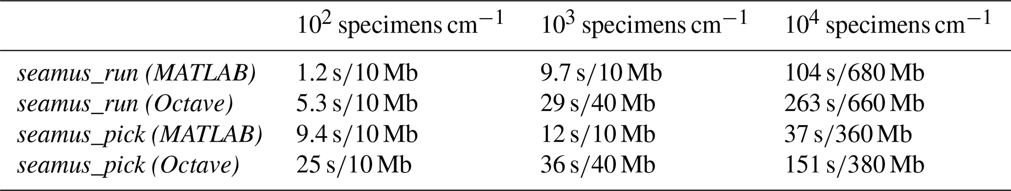
3.2 Processing speed and computing requirements
Where possible, the processing of arrays for simulation time steps has been vectorised (i.e. not processed within an iterative loop), in order to maximise processing speed. For example, the per time step assignment of single-specimen arrays corresponding to ages and carrier signals all occurs within fully vectorised code. However, the bioturbation simulation (i.e. the bioturbation of the assigned depth values) is not vectorised and is carried out within a single-thread iterative loop, due to each iteration of the bioturbation simulation being dependent upon the results of the previous iteration. In order to optimise the processing time on 64-bit computers, all arrays are stored as 64-bit. Should the user wish to save memory, it is possible to select the do32bit option when accessing seamus_run from the command line (see the function documentation). Indicative run times and memory use are shown in Table 1.
The SEAMUS model was developed in MATLAB 2017b and has been tested as compatible with Octave 5.1.0. The seamus_run module can be run using the basic MATLAB environment, with no extra toolboxes. The seamus_pick module runs more efficiently when the Statistics and Machine Learning toolbox (specifically, the prctile function) is installed, but when it is detected that users do not have access to that toolbox, seamus_pick will revert to using a modified version of an equivalent function (Kienzle, 2001), which has been embedded into the script. The seamus_pick function also uses the Matcal (Lougheed and Obrochta, 2016) 14C calibration script, which has been embedded in the SEAMUS download package.
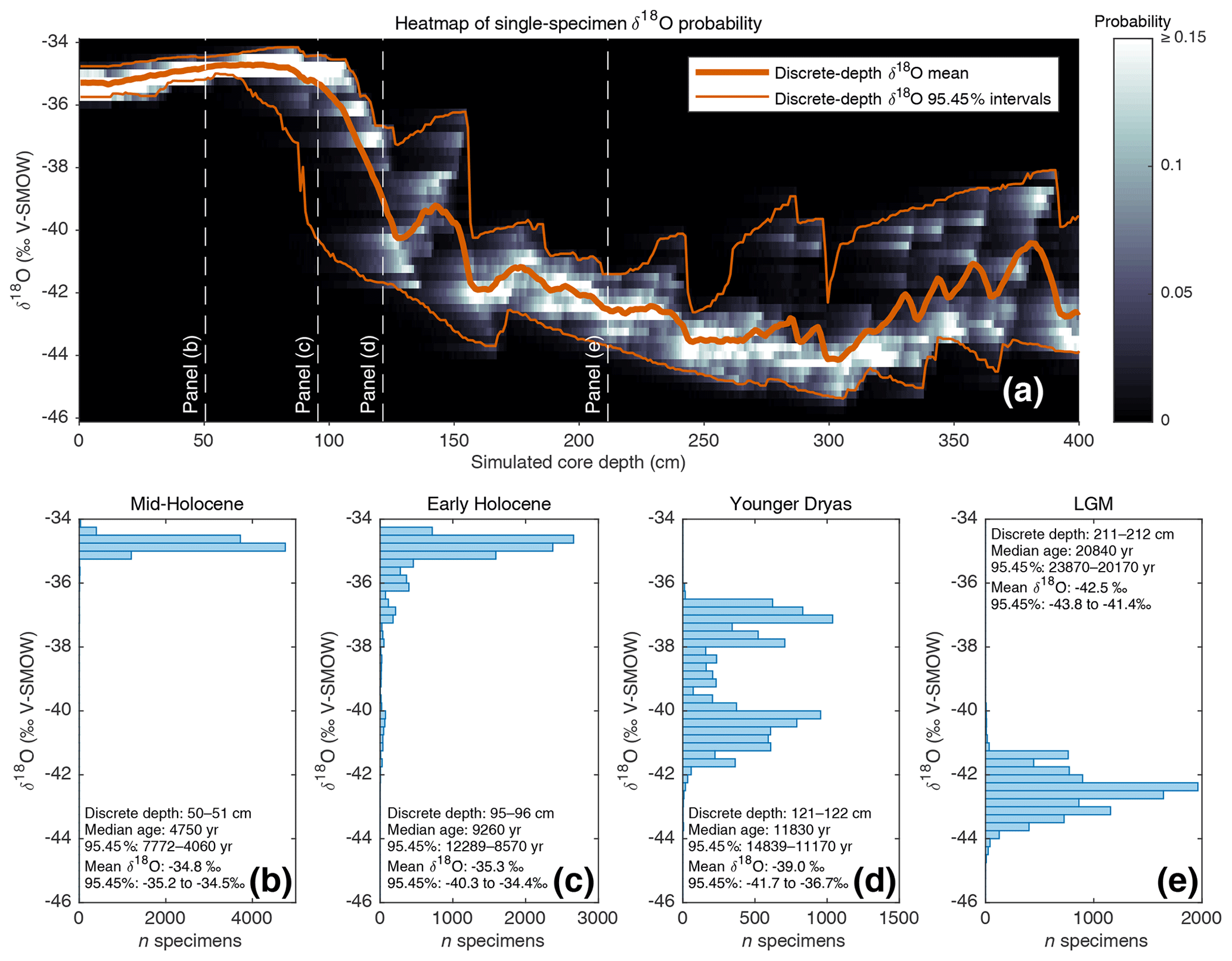
Figure 2(a) Heat map (in greyscale) of downcore single-specimen δ18O value probability. For each 1 cm discrete depth, foraminifera δ18O probability (in 0.25 ‰ bins) is calculated and plotted as a heatmap. Also shown (in orange) are the discrete-depth mean δ18O and corresponding 95.45 % intervals. (b, c, d, e) Single-specimen δ18O histograms for various 1 cm discrete-depth intervals (these discrete depths are also indicated in panel a).
4.1 Analysing downcore specimen population distributions
As outlined in the introduction, advances in stable isotope mass spectrometry have allowed for routine single-specimen analysis, which has led to increased interest in using geochemical analysis of single-specimen populations from discrete depths as a potentially powerful tool with which to reconstruct past changes in climate variability. Such an application tool, however, still relies upon median downcore age by assigning an age estimate to all single specimens from a single depth. Climate variability or seasonality interpretations are clouded, therefore, when single specimens from a wide range of ages are mixed into the same depth, especially if the interpretation relies upon detecting extreme climate events in the form of single-specimen outliers. Using the previously described (Sect. 3.1; Fig. 1b) SEAMUS simulation, it is possible to construct a probability heatmap and 95.45 % intervals for the simulated single-specimen δ18O (Fig. 2a) data. The shape and range of these 95.45 % intervals relative to a glacial–interglacial change is similar to what has been calculated in previous studies (Schiffelbein, 1986), albeit in the case of the Termination II deglaciation. Using SEAMUS, histograms of single-specimen δ18O values for discrete depths can also be explored, for example for sediment core intervals with a median downcore age corresponding to the early Holocene (Fig. 2b), mid-Holocene (Fig. 2c), Younger Dryas (Fig. 2d) and Late Glacial Maximum (Fig. 2e). This analysis demonstrates the potential for the presence of single specimens with glacial climate values being present in samples with an interglacial mean value. For example, in the early Holocene depth interval (Fig. 2c), 15 % of the simulated single specimens have a δ18O value less than or equal to −36 ‰. Of course, some sediment archives may have much higher or lower SAR than the constant 10 cm kyr−1 simulated in this example. The contribution of older specimens to a particular depth interval is dependent upon a number of factors: temporal changes in SAR, BD, species abundance and the susceptibility of older specimens within a discrete depth to be broken and/or dissolved as a consequence of having been through more bioturbation cycles (Rubin and Suess, 1955; Ericson et al., 1956; Emiliani and Milliman, 1966; Barker et al., 2007). Using the SEAMUS model it is possible to run dynamic sediment scenarios to investigate the influence of the mixing of specimens of different ages upon interpretations based upon single-specimen analysis.
4.2 Analysing 14C calibration skill
As outlined earlier, it is possible to assign 14C activities to single specimens in the sedimentation simulation by using suitable records of the Earth's Δ14C history (e.g., IntCal). Subsequently, SEAMUS uses the 14C activities of the specimens contained within each discrete depth to calculate an expected laboratory 14C determination and measurement uncertainty. Using the MatCal software, it is subsequently possible to calibrate the aforementioned 14C age, in combination with a calibration curve and reservoir age estimate, to produce an expected calibrated age distribution. The calibrated age distribution for the discrete depth can be compared with the true age distribution for the discrete depth, as recorded by the simulation, to evaluate the skill with which current 14C dating and calibration processes can reproduce the true age distribution of a particular sediment core slice. A graphical representation of the aforementioned output for a discrete-depth interval is shown in Fig. 3, once again using the SEAMUS bioturbation simulation carried out in Sect. 3.1. This analysis demonstrates that, for the applied simulation parameters and for the discrete-depth interval analysed in Fig. 3 (121–122 cm), the 14C calibration process would produce a median calibrated age of 12.21 cal ka BP, whereas the true median age is 11.79 ka, meaning that there is a 420-year difference between the two. Furthermore, the 14C calibration process produces a 95.45 % credible interval of 12.64–11.65 cal ka BP (a range of 990 cal yr), whereas the true 95.45 % interval of the single specimens within the simulation is 14.95–11.16 ka (a range of 3788 years), meaning that the 14C dating and calibration process considerably underestimates, by some 2800 years, the age uncertainty for this particular interval of simulated sediment core. A MATLAB script enabling users to produce a figure similar to Fig. 3 is included within the tutorial script (tutorial.m) that is bundled with SEAMUS. Users can subsequently explore downcore changes in the effectiveness of 14C dating to accurately estimate true age under various dynamic simulation conditions, including abundance changes, SAR changes, bioturbation depth changes, reservoir age changes, as well as during periods of dynamic Δ14C.
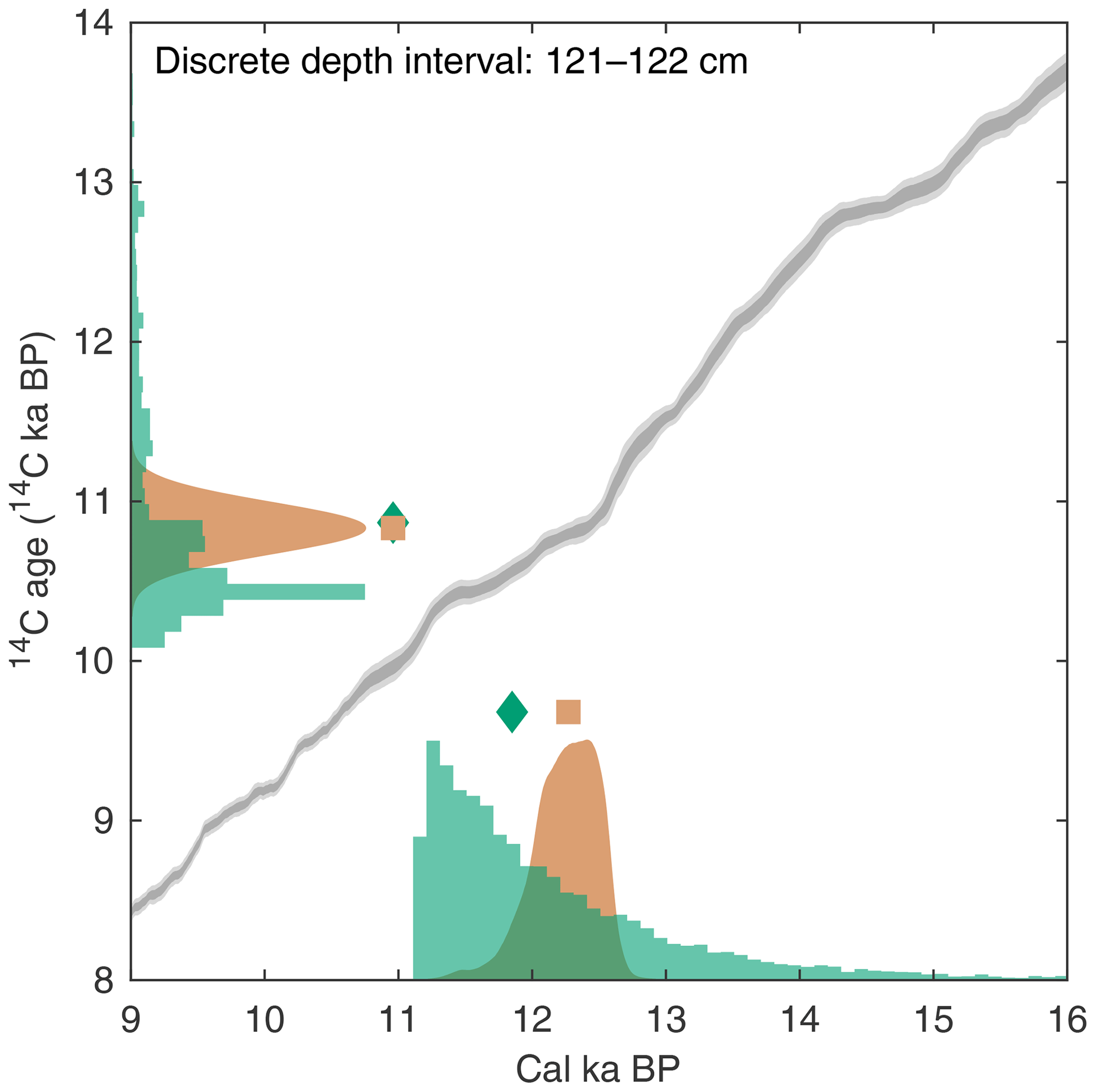
Figure 3Example of using output from a SEAMUS simulation to estimate 14C calibration skill for a particular discrete-depth subsample. The green histograms represent the SEAMUS simulation output: on the x axis the true age distribution of the discrete-depth single specimens (with the green diamond corresponding to the median true age) and on the y axis the 14C age distribution of the single specimens (with the green diamond corresponding to the mean 14C age). All histograms are shown using 100 (14C)-year bins. The orange probability distribution on the y axis represents a normal distribution corresponding to an idealised laboratory 14C analysis of the single specimens, where the orange square corresponds to the expected mean laboratory 14C age. The orange probability distribution on the x axis represents the calibrated age distribution arising from the calibration of the laboratory 14C analysis using Marine13 (Reimer et al., 2013). Also shown, for reference, are the Marine13 calibration curve 1σ (dark grey) and 2σ (light grey) confidence intervals. Simulation output shown in the figure is based on the SEAMUS run in Fig. 1b, with 14C activities assigned to single specimens according to Marine13 with a constant ΔR of 0±0 14C yr. For the picking and calibration, all single specimens within the 121–122 cm discrete depth are picked, and calibration is carried out using MatCal (Lougheed and Obrochta, 2016) with Marine13 and a ΔR of 0±0 14C yr.
4.3 Investigating noise created by the picking process
When picking discrete-depth samples from discrete-depth specimen populations, palaeoceanographers randomly pick whole specimens to produce a downcore mean signal. The seamus_pick module can be used to test for random noise introduced upon the mean signal by the picking process. The module can be repeatedly run with a set number of randomly picked whole specimens per sample, and the resulting picking runs can be compared to an ideal picking run that picks all available whole specimens for each discrete depth. Such an approach is investigated here, once again using the same SEAMUS bioturbation simulation that was carried out in Sect. 3.1, for picking scenarios each with 1 specimen per sample (Fig. 4a), 2 specimens per sample (Fig. 4b), 3 specimens per sample (Fig. 4c), 5 specimens per sample (Fig. 4d), 10 specimens per sample (Fig. 4e) and 20 specimens per sample (Fig. 4f). Such simulations can allow researchers to isolate and quantify the effect of the picking process upon their downcore multi-specimen reconstructions for their particular sediment core scenario. It can be noted that for the 10 cm kyr−1 simulation carried out here, larger sample sizes (n≥10) tend to produce downcore sampling runs close to the total population mean (Fig. 4e and f), although the true spread of values is hidden. Furthermore, even with larger samples sizes there is still the possibility of the generation of picking-noise-induced peak or trough values which could be erroneously interpreted as a precise indication of the timing of a particular climate feature. In the case of very small sample sizes (Fig. 4a and b), researchers can get an idea of the total spread of values within single core intervals. With advances in mass spectrometry making the analysis of single specimens ever more routine and cost-effective, the ideal approach in the future may involve exclusively analysing single specimens, with single-specimen values from discrete depths used to both estimate the signal distribution and calculate a downcore mean signal, thus facilitating a “best of both worlds” approach.
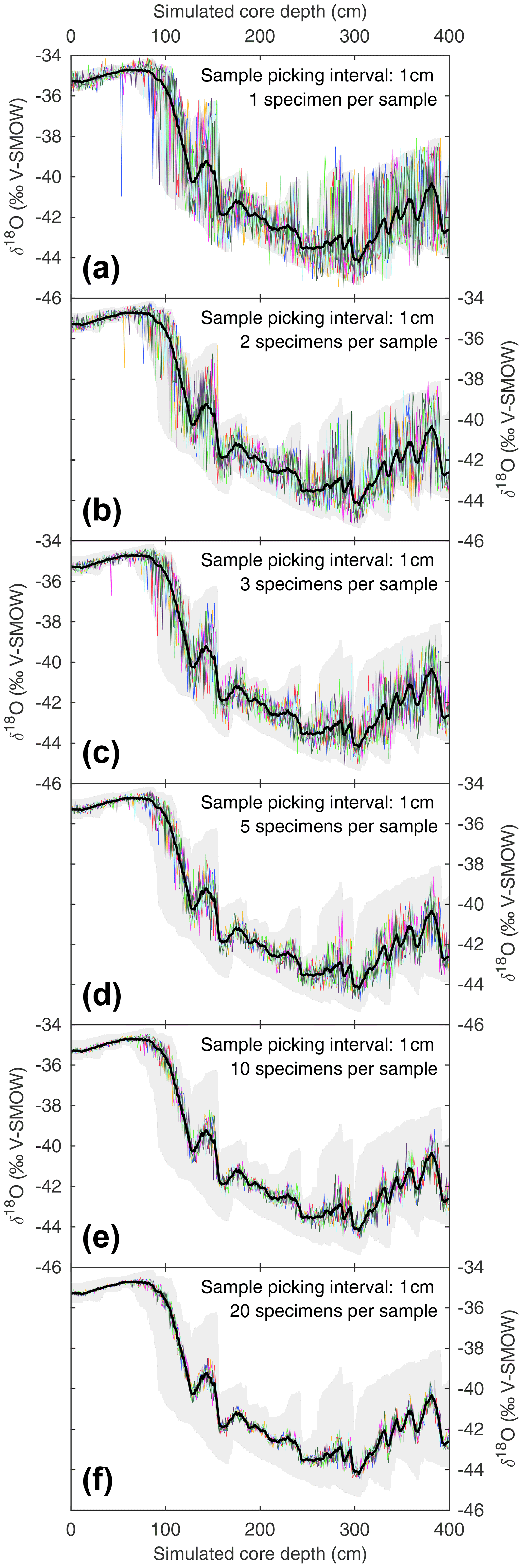
Figure 4Estimating noise induced by subsample size during the picking process. Based on the SEAMUS simulation in Fig. 1b, six sample size scenarios are considered: (a) 1 specimen per sample; (b) 2 specimens per sample; (c) 3 specimens per sample; (d) 5 specimens per sample; (e) 10 specimens per sample; (f) 20 specimens per sample. In each scenario, the downcore picking process is repeated 10 times, and each picking run is represented by a coloured line. Also shown in all panels is the mean δ18O value for all single specimens within discrete-depth intervals (black line) and 95.45 % intervals (filled grey area).
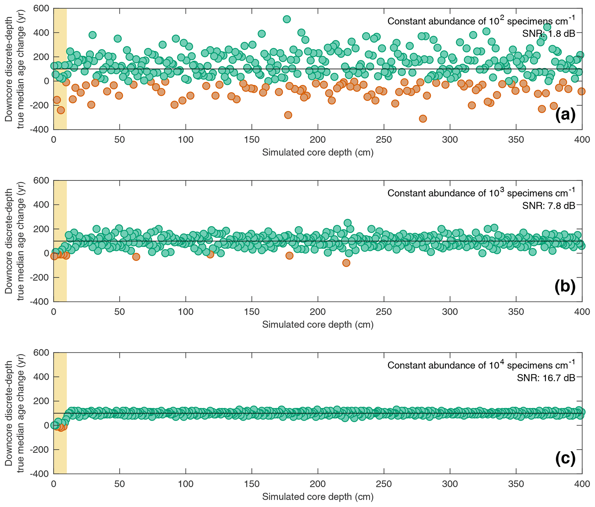
Figure 5Estimating downcore age–depth noise induced by absolute species abundance in three scenarios all involving a constant SAR of 10 cm kyr−1 and constant bioturbation depth of 10 cm. In all three panels, the data points (circles) indicate the downcore discrete-depth median age increase for each centimetre of core depth. Green circles correspond to positive downcore median age change, while orange data points correspond to negative downcore median age change (i.e. apparent age reversals). The horizontal black line in each panel denotes the perfect downcore age change of +100 yr cm−1 that would be associated with a constant SAR of 10 cm kyr−1. The yellow interval denotes the still-active BD (10 cm) at the core top. The signal-to-noise ratio (SNR) is also computed for each scenario as the ratio between the summed squared magnitudes of the signal and of the noise. The still-active BD at the core top is excluded from the SNR calculation. Three different abundance scenarios are shown: (a) constant abundance of 102 specimens cm−1; (b) constant abundance of 103 specimens cm−1; (c) constant abundance of 104 specimens cm−1.

Figure 6Investigating the effect of temporal changes in a species' abundance upon its discrete-depth age–depth signal in the case of a simulated sediment core with a constant SAR of 10 cm kyr−1 and constant BD of 10 cm. In all panels, the yellow interval denotes the still-active BD (10 cm) at the core top. (a) The temporal abundance for a given species “Species A” used in the SEAMUS simulation, inputted into the model as a fraction of the per time step specimen flux. (b) The resulting simulated downcore, discrete-depth (1 cm) absolute abundance (number of specimens) for Species A. Vertical grey bands correspond to the depth of the abundance peaks. (c) The downcore, discrete-depth (1 cm) change in median age based on samples containing only Species A specimens. Green circles denote downcore increase in discrete-depth apparent median age (i.e. positive apparent SAR) and orange circles denote downcore decrease in discrete-depth median age (i.e. apparent age reversals). The horizontal black line in each panel denotes the perfect downcore age change of +100 yr cm−1 that would be associated with a constant SAR of 10 cm kyr−1. (d) The 95.45 % age range of for Species A for each discrete 1 cm depth. (e) The offset between the median age of Species A (MedA) and the median age of all specimens (Medall). Shown in the panel is MedA−Medall. The horizontal black line corresponds to zero (i.e. no offset).
4.4 Investigating noise created by absolute specimen abundance
The interaction between total specimen abundance and bioturbation creates downcore noise in the sedimentary record. In Fig. 5, the downcore, discrete-depth median age increase per centimetre for three SEAMUS simulations, all with an idealised constant SAR of 10 cm kyr−1 and constant BD of 10 cm, is shown, with the number of outputted specimens per centimetre being set differently for each simulation, namely at 102 specimens cm−1 (Fig. 5a), 103 specimens cm−1 (Fig. 5b) and 104 specimens cm−1 (Fig. 5c). In all three scenarios the downcore, discrete-depth increase in median age clusters around 100 yr cm−1, which is what would be expected in the case of a 10 cm kyr−1 sediment core. As expected, the signal-to-noise ratio is higher in cases of higher abundance. An interesting side effect of a decreased signal–noise ratio is the increased likelihood of the generation of apparent age–depth reversals. For example, in the abundance scenario with 102 specimens cm−1 (Fig. 5a), 21.7 % of the discrete-depth (1 cm) age–depth points produce an apparent age–depth reversal. Due to the fact that many age–depth modelling software packages often consider such age–depth reversals as outliers (Blaauw and Christen, 2011; Lougheed and Obrochta, 2019), palaeoceanographers should be aware that the apparent age–depth reversals generated by very noisy downcore signals caused by low specimen abundance may result in age–depth models that are biased towards young ages. Also, while palaeoceanographers often quantify relative abundance as a ratio between different species, it is additionally important to quantify the absolute abundance of a particular species being studied in the form of the number of specimens per specific sediment volume or sample, as this can give clues regarding the expected signal-to-noise ratio ascertained from a discrete-depth analysis.
4.5 Investigating artefacts created by dynamic specimen abundance
In the previous sections, scenarios involving constant specimen abundance were explored. SEAMUS is specifically designed with the ability to process multiple temporally dynamic inputs. In Fig. 6, the effect of temporally dynamic species abundance for a theorised Species A is studied, once again using a scenario with a constant SAR of 10 cm kyr−1 and constant BD of 10 cm. Past studies using simpler mixing models have previously shown that the downcore δ18O signal for particular species can display offsets that are in fact an artefact of the interplay between abundance and bioturbation (Löwemark and Grootes, 2004; Trauth, 2013). Here, the single-specimen SEAMUS simulation is used to investigate the effects of abundance and bioturbation upon the age–depth signal produced by single specimens. In this scenario SEAMUS is driven using a dynamic input with six temporal maxima in Species A specimen flux centred upon 10, 16 18, 28, 32 and 36 ka (Fig. 6a). The resulting post-simulation absolute abundance of Species A in the depth domain (Fig. 6b) is smoothed out as a result of bioturbation. The interaction between dynamic abundance and bioturbation also has consequences for the discrete-depth age–depth relationship of Species A. For example, the downcore change in discrete-depth median age for Species A (Fig. 6c) is less noisy (i.e. less likely to produce outliers) for intervals close to the absolute abundance peaks but is negatively offset from the ideal discrete-depth median age change of 100 yr cm−1 that would be associated with the 10 cm kyr−1 sediment core simulation. This effect would manifest itself in a high depth-resolution age–depth model as an age–depth plateau near to an abundance peak.
Similarly, the 95.45 % discrete-depth age range for Species A is much more constrained in the case of depth intervals located close to the abundance peaks (Fig. 6d) but less representative of the median age for the total sediment (all specimens), with Species A being biased towards ages that are too young (Fig. 6e). This bias is an interesting finding, seeing as it has long been assumed that pooled specimen samples used for dating (e.g. 14C dating) should be retrieved from abundance peaks (Keigwin and Lehman, 1994; Waelbroeck et al., 2001; Galbraith et al., 2015). This assumption is largely based on the fact that 14C dates sampled from abundance peaks are younger than the immediately surrounding sediment (Rafter et al., 2018). However, the SEAMUS simulation suggests that abundance peaks can result in ages that are anomalously young when compared to the total sediment (Fig. 6e).
Deep-sea sediment archives are subject to systematic bioturbation, which can complicate palaeoclimate reconstructions sourced from sediment cores. Complications can include artefacts and/or spurious offsets in 14C age of other carrier signals (such as δ18O) sourced from multi-specimen samples. The SEAMUS model allows users to interactively investigate how such artefacts and/or spurious offsets can be attributed to the mixing of single specimens. The model is suitable for users who are investigating the downcore mean signal and how it is affected by dynamic changes in input variables. The model is especially interesting for researchers who are using single-specimen foraminifera analysis to quantify past changes in seasonality or multi-centennial amplitude in regional climate variability, as it can assist researchers in understanding the influence of bioturbation upon their results and interpretation. Users can also consider combining the model with proxy and ecological models to attain a total picture of sediment archive climate reconstructions. The model is also useful as a teaching resource; for example, users can keep all but one input variable constant and learn to understand the influence of dynamic changes in that particular input variable upon the downcore specimen record. Subsequently, multiple dynamic variables can be introduced into the mix, allowing for an incremental learning experience.
The latest release version of the SEAMUS model and accompanying interactive tutorial (for both MATLAB and Octave) can be downloaded from the Zenodo public repository (https://doi.org/10.5281/zenodo.3251654, Lougheed, 2019). The Zenodo repository also contains a link to SEAMUS on Github (https://github.com/bryanlougheed/seamus).
The author declares that there is no conflict of interest.
Thanks to Laboratoire d'Océanologie et de Géosciences for kindly hosting me as a guest researcher at Université du Littoral Côte d'Opal. Brett Metcalfe is thanked for various discussions about the state-of-the-art of single-specimen foraminifera analysis (see also the resources at http://www.brett-metcalfe.com, last access: 15 January 2019). Two anonymous reviewers are thanked for their helpful input.
This research has been supported by the Swedish Research Council (Vetenskapsrådet; grant no. 2018-04992).
This paper was edited by Paul Halloran and reviewed by two anonymous referees.
Bard, E., Arnold, M., Duprat, J., Moyes, J., and Duplessy, J. C.: Reconstruction of the last deglaciation: Deconvolved records of δ18O profiles, micropaleontological variations and accelerator mass spectrometric 14C dating, Clim. Dynam., 1, 101–112, 1987.
Barker, S., Broecker, W., Clark, E., and Hajdas, I.: Radiocarbon age offsets of foraminifera resulting from differential dissolution and fragmentation within the sedimentary bioturbated zone, Paleoceanography, 22, PA2205, https://doi.org/10.1029/2006PA001354, 2007.
Berger, W. H. and Heath, G. R.: Vertical mixing in pelagic sediments, J. Mar. Res., 26, 134–143, 1968.
Berger, W. H. and Johnson, R. F.: On the thickness and the 14C age of the mixed layer in deep-sea carbonates, Earth Planet. Sc. Lett., 41, 223–227, 1978.
Berger, W. H. and Killingley, J. S.: Box cores from the equatorial Pacific: 14C sedimentation rates and benthic mixing, Mar. Geol., 45, 93–125, https://doi.org/10.1016/0025-3227(82)90182-7, 1982.
Billups, K. and Spero, H. J.: Reconstructing the stable isotope geochemistry and paleotemperatures of the equatorial Atlantic during the last 150,000 years: Results from individual foraminifera, Paleoceanography, 11, 217–238, https://doi.org/10.1029/95PA03773, 1996.
Blaauw, M. and Christen, J. A.: Flexible Paleoclimate Age-Depth Models Using an Autoregressive Gamma Process, Bayesian Anal., 6, 457–474, https://doi.org/10.1214/11-BA618, 2011.
Boudreau, B. P.: Mean mixed depth of sediments: The wherefore and the why, Limnol. Oceanogr., 43, 524–526, https://doi.org/10.4319/lo.1998.43.3.0524, 1998.
Dolman, A. M. and Laepple, T.: Sedproxy: a forward model for sediment-archived climate proxies, Clim. Past, 14, 1851–1868, https://doi.org/10.5194/cp-14-1851-2018, 2018.
Emiliani, C. and Milliman, J. D.: Deep-sea sediments and their geological record, Earth-Sci. Rev., 1, 105–132, https://doi.org/10.1016/0012-8252(66)90002-X, 1966.
Ericson, D. B., Broecker, W. S., Kulp, J. L., and Wollin, G.: Late-Pleistocene Climates and Deep-Sea Sediments, Science, 124, 385–389, https://doi.org/10.1126/science.124.3218.385, 1956.
Ford, H. L. and Ravelo, A. C.: Estimates of Pliocene Tropical Pacific Temperature Sensitivity to Radiative Greenhouse Gas Forcing, Paleoceanography and Paleoclimatology, 34, 2–15, https://doi.org/10.1029/2018PA003461, 2019.
Ford, H. L., Ravelo, A. C., and Polissar, P. J.: Reduced El Nino-Southern Oscillation during the Last Glacial Maximum, Science, 347, 255–258, https://doi.org/10.1126/science.1258437, 2015.
Fraass, A. J. and Lowery, C. M.: Defining uncertainty and error in planktic foraminiferal oxygen isotope measurements: Uncertainty in Foram Oxygen Isotopes, Paleoceanography, 32, 104–122, https://doi.org/10.1002/2016PA003035, 2017.
Galbraith, E. D., Kwon, E. Y., Bianchi, D., Hain, M. P., and Sarmiento, J. L.: The impact of atmospheric CO2 on carbon isotope ratios of the atmosphere and ocean, Global Biogeochem. Cy., 29, 307–324, https://doi.org/10.1002/2014GB004929, 2015.
Ganssen, G. M., Peeters, F. J. C., Metcalfe, B., Anand, P., Jung, S. J. A., Kroon, D., and Brummer, G.-J. A.: Quantifying sea surface temperature ranges of the Arabian Sea for the past 20 000 years, Clim. Past, 7, 1337–1349, https://doi.org/10.5194/cp-7-1337-2011, 2011.
Ho, S. L., Mollenhauer, G., Fietz, S., Martínez-Garcia, A., Lamy, F., Rueda, G., Schipper, K., Méheust, M., Rosell-Melé, A., Stein, R., and Tiedemann, R.: Appraisal of TEX86 and TEX86L thermometries in subpolar and polar regions, Geochim. Cosmochim. Ac., 131, 213–226, https://doi.org/10.1016/j.gca.2014.01.001, 2014.
Keigwin, L. D. and Lehman, S. J.: Deep circulation change linked to HEINRICH Event 1 and Younger Dryas in a middepth North Atlantic Core, Paleoceanography, 9, 185–194, https://doi.org/10.1029/94PA00032, 1994.
Kienzle, P.: Octave prctile() function, available at: https://sourceforge.net/p/octave/statistics/ci/c1ef33a337b30168a0581d9cae26397d2c1ae06a/tree/inst/prctile.m#l28 (last access: 20 April 2019), 2001.
Killingley, J. S., Johnson, R. F. and Berger, W. H.: Oxygen and carbon isotopes of individual shells of planktonic foraminifera from Ontong-Java plateau, equatorial pacific, Palaeogeogr. Palaeocl., 33, 193–204, https://doi.org/10.1016/0031-0182(81)90038-9, 1981.
Lombard, F., Labeyrie, L., Michel, E., Bopp, L., Cortijo, E., Retailleau, S., Howa, H., and Jorissen, F.: Modelling planktic foraminifer growth and distribution using an ecophysiological multi-species approach, Biogeosciences, 8, 853–873, https://doi.org/10.5194/bg-8-853-2011, 2011.
Lougheed, B. C.: SEAMUS (v 1.20) SEdiment AccuMUlation Simulator (Version 1.20), Zenodo, https://doi.org/10.5281/zenodo.3558292, 2019.
Lougheed, B. C. and Obrochta, S. P.: MatCal: Open Source Bayesian 14C Age Calibration in Matlab, J. Open Res. Softw., 4, e42, https://doi.org/10.5334/jors.130, 2016.
Lougheed, B. C. and Obrochta, S. P.: A rapid, deterministic age-depth modelling routine for geological sequences with inherent depth uncertainty, Paleoceanography and Paleoclimatology, 34, 122–133, https://doi.org/10.1029/2018PA003457, 2019.
Lougheed, B. C., Metcalfe, B., Ninnemann, U. S., and Wacker, L.: Moving beyond the age–depth model paradigm in deep-sea palaeoclimate archives: dual radiocarbon and stable isotope analysis on single foraminifera, Clim. Past, 14, 515–526, https://doi.org/10.5194/cp-14-515-2018, 2018.
Löwemark, L. and Grootes, P. M.: Large age differences between planktic foraminifers caused by abundance variations and Zoophycos bioturbation, Paleoceanography, 19, PA2001, https://doi.org/10.1029/2003PA000949, 2004.
Metcalfe, B., Feldmeijer, W., de Vringer-Picon, M., Brummer, G.-J. A., Peeters, F. J. C., and Ganssen, G. M.: Late Pleistocene glacial–interglacial shell-size–isotope variability in planktonic foraminifera as a function of local hydrography, Biogeosciences, 12, 4781–4807, https://doi.org/10.5194/bg-12-4781-2015, 2015.
Metcalfe, B., Lougheed, B. C., Waelbroeck, C., and Roche, D. M.: On the validity of foraminifera-based ENSO reconstructions, Clim. Past Discuss., https://doi.org/10.5194/cp-2019-9, in review, 2019a.
Metcalfe, B., Feldmeijer, W., and Ganssen, G. M.: Oxygen Isotope Variability of Planktonic Foraminifera Provide Clues to Past Upper Ocean Seasonal Variability, Paleoceanography and Paleoclimatology, 34, 374–393, https://doi.org/10.1029/2018PA003475, 2019b.
North Greenland Ice Core Project members: High-resolution record of Northern Hemisphere climate extending into the last interglacial period, Nature, 431, 147–151, https://doi.org/10.1038/nature02805, 2004.
Peng, T.-H., Broecker, W. S., and Berger, W. H.: Rates of benthic mixing in deep-sea sediment as determined by radioactive tracers, Quaternary Res., 11, 141–149, 1979.
Pisias, N. G.: Geologic time series from deep-sea sediments: Time scales and distortion by bioturbation, Mar. Geol., 51, 99–113, 1983.
Rafter, P. A., Herguera, J.-C., and Southon, J. R.: Extreme lowering of deglacial seawater radiocarbon recorded by both epifaunal and infaunal benthic foraminifera in a wood-dated sediment core, Clim. Past, 14, 1977–1989, https://doi.org/10.5194/cp-14-1977-2018, 2018.
Rasmussen, S. O., Bigler, M., Blockley, S. P., Blunier, T., Buchardt, S. L., Clausen, H. B., Cvijanovic, I., Dahl-Jensen, D., Johnsen, S. J., Fischer, H., Gkinis, V., Guillevic, M., Hoek, W. Z., Lowe, J. J., Pedro, J. B., Popp, T., Seierstad, I. K., Steffensen, J. P., Svensson, A. M., Vallelonga, P., Vinther, B. M., Walker, M. J. C., Wheatley, J. J., and Winstrup, M.: A stratigraphic framework for abrupt climatic changes during the Last Glacial period based on three synchronized Greenland ice-core records: refining and extending the INTIMATE event stratigraphy, Quaternary Sci. Rev., 106, 14–28, https://doi.org/10.1016/j.quascirev.2014.09.007, 2014.
Reimer, P. J., Bard, E., Bayliss, A., Beck, J. W., Blackwell, P. G., Ramsey, C. B., Buck, C. E., Cheng, H., Edwards, R. L., Friedrich, M., Grootes, P. M., Guilderson, T. P., Haflidason, H., Hajdas, I., Hatté, C., Heaton, T. J., Hoffmann, D. L., Hogg, A. G., Hughen, K. A., Kaiser, K. F., Kromer, B., Manning, S. W., Niu, M., Reimer, R. W., Richards, D. A., Scott, E. M., Southon, J. R., Staff, R. A., Turney, C. S. M., and van der Plicht, J.: IntCal13 and Marine13 Radiocarbon Age Calibration Curves 0–50,000 Years cal BP, Radiocarbon, 55, 1869–1887, 2013.
Roche, D. M.: δ18O water isotope in the iLOVECLIM model (version 1.0) – Part 1: Implementation and verification, Geosci. Model Dev., 6, 1481–1491, https://doi.org/10.5194/gmd-6-1481-2013, 2013.
Roche, D. M., Waelbroeck, C., Metcalfe, B., and Caley, T.: FAME (v1.0): a simple module to simulate the effect of planktonic foraminifer species-specific habitat on their oxygen isotopic content, Geosci. Model Dev., 11, 3587–3603, https://doi.org/10.5194/gmd-11-3587-2018, 2018.
Rubin, M. and Suess, H. E.: U.S. Geological Survey Radiocarbon Dates 11, Science, 121, 481–488, 1955.
Schiffelbein, P.: Effect of benthic mixing on the information content of deep-sea stratigraphical signals, Nature, 311, 651, https://doi.org/10.1038/311651a0, 1984.
Schiffelbein, P.: The interpretation of stable isotopes in deep-sea sediments: An error analysis case study, Mar. Geol., 70, 313–320, https://doi.org/10.1016/0025-3227(86)90008-3, 1986.
Seierstad, I. K., Abbott, P. M., Bigler, M., Blunier, T., Bourne, A. J., Brook, E., Buchardt, S. L., Buizert, C., Clausen, H. B., Cook, E., Dahl-Jensen, D., Davies, S. M., Guillevic, M., Johnsen, S. J., Pedersen, D. S., Popp, T. J., Rasmussen, S. O., Severinghaus, J. P., Svensson, A., and Vinther, B. M.: Consistently dated records from the Greenland GRIP, GISP2 and NGRIP ice cores for the past 104 ka reveal regional millennial-scale δ18O gradients with possible Heinrich event imprint, Quaternary Sci. Rev., 106, 29–46, https://doi.org/10.1016/j.quascirev.2014.10.032, 2014.
Spero, H. J. and Williams, D. F.: Evidence for seasonal low-salinity surface waters in the Gulf of Mexico over the last 16,000 years, Paleoceanography, 5, 963–975, https://doi.org/10.1029/PA005i006p00963, 1990.
Tang, C. M. and Stott, L. D.: Seasonal salinity changes during Mediterranean sapropel deposition 9000 years B.P.: Evidence from isotopic analyses of individual planktonic foraminifera, Paleoceanography, 8, 473–493, https://doi.org/10.1029/93PA01319, 1993.
Thirumalai, K., Partin, J. W., Jackson, C. S., and Quinn, T. M.: Statistical constraints on El Niño Southern Oscillation reconstructions using individual foraminifera: A sensitivity analysis: IFA-ENSO UNCERTAINTY, Paleoceanography, 28, 401–412, https://doi.org/10.1002/palo.20037, 2013.
Tierney, J. E. and Tingley, M. P.: A TEX 86 surface sediment database and extended Bayesian calibration, Sci. Data, 2, 1–10, https://doi.org/10.1038/sdata.2015.29, 2015.
Tierney, J. E., Malevich, S. B., Gray, W., Vetter, L., and Thirumalai, K.: Bayesian calibration of the Mg/Ca paleothermometer in planktic foraminifera, Paleoceanography and Paleoclimatology, https://doi.org/10.1029/2019PA003744, online first, 2019.
Trauth, M. H.: TURBO: a dynamic-probabilistic simulation to study the effects of bioturbation on paleoceanographic time series, Comput. Geosci., 24, 433–441, https://doi.org/10.1016/S0098-3004(98)00019-3, 1998.
Trauth, M. H.: TURBO2: A MATLAB simulation to study the effects of bioturbation on paleoceanographic time series, Comput. Geosci., 61, 1–10, https://doi.org/10.1016/j.cageo.2013.05.003, 2013.
Trauth, M. H., Sarnthein, M., and Arnold, M.: Bioturbational mixing depth and carbon flux at the seafloor, Paleoceanography, 12, 517–526, 1997.
Waelbroeck, C., Duplessy, J.-C., Michel, E., Labeyrie, L., Paillard, D., and Duprat, J.: The timing of the last deglaciation in North Atlantic climate records, Nature, 412, 724–727, 2001.
Wit, J. C., Reichart, G. J., and Ganssen, G. M.: Unmixing of stable isotope signals using single specimen δ18O analyses, Geochem. Geophy. Geosy., 14, 1312–1320, https://doi.org/10.1002/ggge.20101, 2013.