2.1 Model architecture

AtChem was initially developed as a web application to provide a modelling tool for laboratory and environmental chamber studies that could be used by both experienced and novice users, particularly within the EUROCHAMP community. The original version, which will be referred to as AtChem-online in this paper, is compiled and run on a dedicated web server and can be used with just a text editor, file compression software, a web browser and an internet connection. AtChem-online (version 1.5, rev. 146) is accessible at https://atchem.leeds.ac.uk/webapp/, with a simple tutorial available at http://mcm.york.ac.uk/atchem/tutorial_intro.htt (last access: 16 January 2020): the user simply needs to provide the chemical mechanism, the configuration files and the model parameters via a web form. The model results are stored on the web server and can be downloaded as compressed zip files for further processing and analysis.

While relatively simple and easy to use, AtChem-online has a number of limitations, mostly related to its nature as a web application. It cannot be customised by a user beyond what the Web interface allows, and, more importantly, it cannot be used for batch model runs – i.e. multiple runs of the same model with minor and/or incremental modifications, a modelling approach which is very useful for sensitivity studies. Moreover, the models required for ambient measurements and field campaigns are often more complex than those required for environmental chambers and laboratory experiments and need to be run for longer periods of time (several hours or days). Such models can be computationally very expensive and are therefore difficult to run from a web server with limited resources.

AtChem2 was developed from AtChem-online to overcome these limitations. The aim of AtChem2 was to create an offline version of AtChem capable of running long simulations of computationally intensive models and to make it possible to run batch simulations. Version 1.0 of AtChem2 (https://doi.org/10.5281/zenodo.3404021, Sommariva and Cox, 2017) is presented here, and it has been used for the model simulations shown in Sect. 3. Although the code base has been extensively reworked, the basic architectures of AtChem-online and AtChem2 are very similar (Fig. 1). The structure and functions of AtChem are organised into five independent components, plus the chemical mechanism which is provided externally (Sect. 2.2):

• Web interface includes the graphical user interface of AtChem-online, accessible via a web browser. In AtChem2, which does not run as a web application, this component has been removed.

• Configuration layer includes the initial conditions, model constraints, input and output variables, and model and solver parameters.

• Processing layer includes the conversion of the chemical mechanism into Fortran format, sum of organic peroxy radicals (RO₂), and parameterisation of photolysis rates.

• Logic layer includes the conversion of the chemical mechanism and of the model configuration into a system of coupled ODEs and boundary conditions of the ODE system.

• Mathematical layer includes the interpolation of constrained variables and integration of the ODE system.

Most of the AtChem code base is written in Fortran 90/95; Python and shell scripts are used in the Web interface, the Processing layer and the Configuration layer. The source code of AtChem-online is available at https://atchem.leeds.ac.uk/sources/ (last access: 16 January 2020), and the source code and the documentation of AtChem2 are available at https://github.com/AtChem/ under the open-source MIT License. AtChem2 can be installed on a Unix/Linux or macOS machine and requires the user to have an elementary knowledge of the Unix command line. Installation of AtChem2 (and of its dependencies) is semi-automated via a number of well-documented scripts that require minimal input from the user. The compilation of AtChem2, which is also done via a script, creates an executable file which reads the configuration of the model at runtime from a directory chosen by the user. For both versions of AtChem, the model configuration – including inputs, outputs and constrained variables – is set via simple text files, which can be modified with a normal text editor. In AtChem2 the configuration files are stored in a dedicated directory, while in AtChem-online they need to be uploaded (together with the chemical mechanism) to the web server.

Figure 1Structure of the AtChem model. The dashed lines indicate the model components that are present in AtChem-online, but not in AtChem2.

Download

The AtChem-online code base (rev. 146) was the starting point for the development of AtChem2. Several parts of the code were modified: the web tools were removed and the code was reorganised into Fortran modules, thoroughly commented and partially rewritten to fully conform to the Fortran 90/95 standard. An important addition to AtChem2 is the implementation of a continuous integration workflow for the development of the model coupled with an extensive suite of tests, which means that every change to the source code is automatically checked against previous model results before being accepted into the code base. In recent years, continuous integration and testing have become standard practice in the software industry, allowing programmers to quickly detect bugs and errors, to ensure that modifications to the code do not result in unintended behaviour and to improve the overall quality of the code. The suite of tests in AtChem2 includes unit tests of individual model functions and complete model runs: it is designed to cover a significant percentage of the code base (∼90 %) and a wide range of common model configurations. Together with the use of the open-source version control software git (https://git-scm.com/, last access: 16 January 2020), these modern software development practices make the AtChem2 model easy to maintain, robust and reliable, and fully traceable and reproducible.

2.2 Chemical mechanism

AtChem is designed to use the Master Chemical Mechanism (MCM) as its chemical mechanism. The entire MCM, or a subset of it, can be downloaded from the MCM website in a variety of formats using the online extraction tool (http://mcm.york.ac.uk/extract.htt, last access: 16 January 2020). The current version of AtChem requires the chemical mechanism to be provided in a format compatible with the one used by FACSIMILE (Curtis and Sweetenham, 1987), a common commercial software for modelling the kinetics of chemical and physical systems (MCPA Software Ltd., UK). The advantage of this format to describe a chemical mechanism is that it is simple and easy to read and modify. A chemical reaction is defined using the following notation:

% k : R1 + R2 = P1 + P2 ;

where k is the rate coefficient, R1 and R2 are the reactants, and P1 and P2 are the products. Chemical reactions can also be written without reactants or products, which is useful to parameterise non-chemical processes in the model, if required. For example, emission of species P1 can be parameterised as

% Er : = P1 ;

where Er is the emission rate in reciprocal seconds (s⁻¹). Likewise, dry deposition and dilution of species R1 can be parameterised, respectively, as

% Vd/BLHEIGHT : R1 = ;
% DILUTE : R1 = ;

where Vd is the deposition velocity in centimetres per second (cm s⁻¹), BLHEIGHT is the boundary layer height in centimetres (cm) and DILUTE is the dilution rate in reciprocal seconds (s⁻¹). BLHEIGHT and DILUTE are environment variables (Sect. 2.3), and they can be set to a value chosen by the user or constrained to prescribed values.

The chemical mechanism file extracted from the MCM website does not need to be modified in order to be used in AtChem. A chemical mechanism different from the MCM can be used, provided that it is in the correct format and it follows the requirements of the MCM. In particular, the calculation of photolysis rates and the sum of organic peroxy radicals (RO₂) must be treated as described in the MCM protocol papers (Jenkin et al., 1997; Saunders et al., 2003). These aspects of the AtChem model are further discussed in Sects. 2.3 and 2.4.

In order to create the executable file, the chemical mechanism needs to be converted into a format readable by the Fortran compiler, a task performed by a series of Python and shell scripts during the build process (Sect. 2.5). In AtChem-online the conversion is done once the user has uploaded the chemical mechanism file (with the configuration files) to the web server via the Web interface, while in AtChem2 the user simply needs to execute a shell script and give the name and path of the chemical mechanism file (Fig. 1). The chemical mechanism is the only part of the model that needs to be compiled with the Fortran source code: all the configuration files (inputs, outputs, constraints, model and solver parameters) are read into the model at runtime, meaning that changes in the model configuration do not require the model to be recompiled (Sect. 2.5).

2.3 Variables and constraints

AtChem, and the MCM, have three types of variables:

• Chemical species include atoms and molecules in the chemical mechanism. The exceptions are CO₂, which, as an end product of VOC oxidation, is not considered by the MCM, and H₂O, which is an environment variable (see below); molecular oxygen and nitrogen (O₂ and N₂) are treated as model parameters and their concentrations are calculated from temperature and pressure. A special chemical variable is RO2, the sum of all the organic peroxy radicals, which is calculated at runtime by the model using the complete list of organic peroxy radicals in the MCM. RO2 is a key element of the MCM protocol – an approximation designed to reduce the number of peroxy radical self and cross reactions (Jenkin et al., 1997). The list of organic peroxy radicals can be empty if a mechanism other than the MCM is used, in which case RO2 has a value of zero.

• Environment variables include physical characteristics of the model, such as temperature, pressure and solar angles (sun declination, solar zenith angle). Water (H₂O), which can be calculated from relative humidity, is considered an environment variable, not a chemical species. Additional environment variables allow the user to apply a scaling factor to the photolysis rates (JFAC, Sect. 2.4) and to use specific parameters for ambient studies (e.g. boundary layer height) or for environmental chamber experiments (e.g. chamber dilution, roof open/closed).

• Photolysis rates include reaction rates of the photolysis reactions in the chemical mechanism. The treatment of photolysis rates in the model is described in detail in Sect. 2.4.

All chemical species, most environment variables and all the photolysis rates can be constrained to prescribed values, such as ambient or chamber measurements. When a variable is constrained, the solver is forced to use its value at each time step to calculate the values of the other variables. The constrained data are stored as simple text files in the corresponding directories.

Table 1Frequencies of the original measurements and averaged frequencies of the constrained data used in each model scenario.

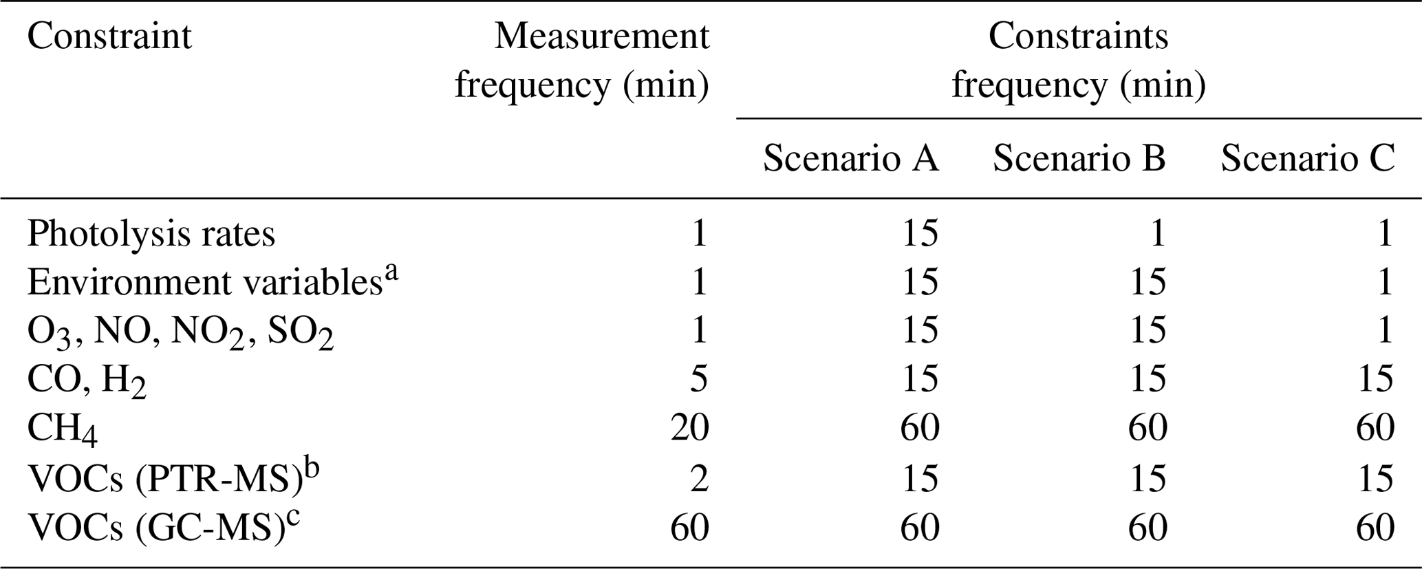
^a temperature, pressure, relative humidity, sun declination. ^b C₁–C₄ oxygenated hydrocarbons. ^c C₂–C₇ hydrocarbons.

Download Print Version | Download XLSX

Constrained box models are often used to study the chemical processes in a given location (e.g. where a field campaign has taken place) or in a chamber experiment. The rationale behind this modelling approach is that short-lived reactive species are not significantly affected by atmospheric transport or other physical processes. Radical species – such as OH, HO₂, RO₂ and, under certain conditions, NO₃ (Brown et al., 2003; Sommariva et al., 2009) – have lifetimes between a few seconds to a few minutes. Therefore, the in situ concentrations of radicals can be calculated from the measured concentrations of longer-lived species and from the measurements of other parameters (photolysis rates, temperature, pressure, etc.). Hence, the ability of the model to reproduce the observations of radical species is an effective test of the description of atmospheric chemical processes in the model (Eisele et al., 1994; Carslaw et al., 1999). The main problem of this modelling technique is that the datasets of constrained variables are often provided with different time frequencies, depending on the instrument or analytical technique used for the measurement. Some species (e.g. O₃, NO, NO₂) are usually measured once every minute, while others (e.g. most VOCs measured by gas chromatography) are typically measured once every 30–60 min. Additionally, data from some instruments may be missing for short periods of time, due to operational limitations, calibrations or instrument downtime. A common method to address this issue is to average the constraints to the lowest time frequency available (e.g. 30 min). However, this introduces significant uncertainties in the model results and does not allow investigations of the short-scale changes in atmospheric composition (Sonderfeld et al., 2016).

An alternative approach is to interpolate the model constraints to fill the gaps and compensate for the different timescales. In AtChem, each constraint is separately interpolated at runtime, using piecewise linear interpolation (piecewise constant interpolation is also available). The advantage of using an interpolation method is that setting up the model is easier and faster, as there is no need to average the constrained data onto a single time base beforehand. More importantly, the constrained data can be used with the original time frequency, thus retaining the important kinetic and mechanistic information that is lost by averaging to the lowest time frequency (Sonderfeld et al., 2016). The disadvantage is that some assumptions are made about the time evolution of the low-frequency constraints, which may lead to serious errors if, for example, the gaps in the data are large or the short-term variability is high.

The impact of the frequency of the constrained data on the model results was investigated using an AtChem2 model constrained to the measurements of 32 chemical species, 18 photolysis rates and 4 environment variables. The frequencies of the measurements are shown in Table 1. Three model scenarios were used: in all scenarios, methane and C₂–C₇ hydrocarbons were averaged to 60 min, while C₁–C₄ oxygenated hydrocarbons, CO and H₂ were averaged to 15 min. In scenario A, the photolysis rates; the environment variables; and the chemical species O₃, NO, NO₂, and SO₂ were averaged to 15 min. Scenario B was identical to scenario A except the photolysis rates were not averaged but used with the original measurement frequency (1 min). Scenario C was identical to scenario B except the environment variables and the chemical species O₃, NO, NO₂, SO₂ were not averaged but used with the original measurement frequency (1 min).

The model was run for 9 d, with a 12 h spin-up period in order to get short-lived intermediates into steady state: as explained above, AtChem interpolated the constrained data at runtime where necessary. The relative differences between the modelled concentrations of a target species (e.g. OH or HO₂) in each scenario were calculated with Eq. (2):

where X_i is the concentration of the target species in scenario i and X_A is the concentration of the target species in the reference scenario (A). Scenario A was used as reference because averaging all measured data to 15 min is common practice for constrained models; OH and HO₂ were chosen as target species because of their central role in this type of modelling study, as explained above. Figure 2 shows the diurnal distributions of the median relative differences, binned by hour of the day, for the 9 d model run.

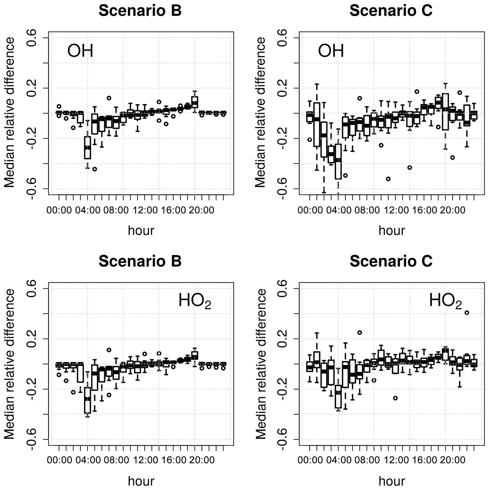
Figure 2Diurnal distributions of the relative differences in the calculated concentrations of OH and HO₂ in scenarios B and C compared to scenario A (Table 1) over a 9 d model run. The box-and-whiskers plots show the medians and the 1st and 3rd quartiles, while the open circles indicate the outliers.

Download

Figure 3Treatment of photolysis rates in AtChem.

Download

The model constrained to 1 min photolysis rates (scenario B) calculated higher concentrations of OH and HO₂ (10 %–15 % in the morning and ∼5 % in the afternoon) compared to the model constrained to 15 min photolysis rates (scenario A). Increasing the frequency of the chemical species O₃, NO, NO₂, and SO₂ and of the environment variables (scenario C) resulted in even larger changes in the calculated concentrations of OH and HO₂ at all times of the day, with variations of up to 20 % for OH and up to 15 % for HO₂. In both scenarios B and C, the differences in the calculated radical concentrations were higher (up to 40 % relative to scenario A) during sunrise and sunset than during the rest of the day (Fig. 2). These periods are critical for a model from a chemical and mathematical point of view, because they correspond to the sharp changes in the atmospheric chemical processes caused by the photochemical reactions starting and stopping. These discontinuities typically result in increased stiffness of the ODE system (Sect. 2.6), leading to larger uncertainties in the calculations.

Figure 2 shows that the frequency of the constrained variables has a significant effect on the model results, especially during sunrise and sunset. The interpolation of constraints allows the model to use as many high-frequency data as are available, resulting in more precise, if not more accurate, model results. It must be noted that the use of high-frequency data as model constraints has the downside of slowing down the integration of the model. For example, the model runtime for scenario C is approximately 20 %–30 % longer than for scenario A. It is up to the user to decide on the balance between model precision and model runtime, depending on the objectives of the modelling work and on the available computing resources.

2.4 Photolysis rates

AtChem implements the parameterisation used by the MCM to calculate the photolysis rates of the appropriate chemical species under clear-sky conditions (Jenkin et al., 1997; Saunders et al., 2003). Each photolysis rate (j) is calculated with Eq. (3):

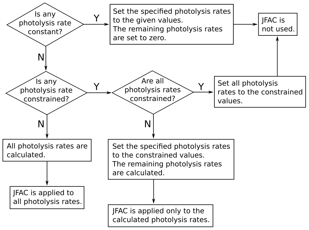
where l, m, and n are empirical parameters; SZA is the solar zenith angle; and τ is a transmission factor. The empirical parameters l, m, n are calculated, for each version of the MCM, as explained by Jenkin et al. (1997) and Saunders et al. (2003): in the MCM v3.3.1 (and previous versions), the empirical parameters are obtained by fitting Eq. (3) to the output of a two-stream isotropic scattering model, which incorporates the appropriate photolysis cross-sections and quantum yields. The transmission factor τ can be used to account for the loss of natural or artificial light in some environmental chambers caused, for example, by the transmittance of the chamber walls (by default, τ=1). In AtChem2, the user can customise the photolysis rates parameterisation by providing an alternative file to replace the values of l, m, n and τ provided by the MCM. The solar zenith angle (SZA) is calculated by AtChem from latitude, longitude, day of the year, time of the day and sun declination according to Madronich (1993). The photolysis rates can also be set to constant values, constrained to measured data or constrained to values calculated offline using a suitable radiative transfer model: the flowchart in Fig. 3 shows how AtChem combines constant, calculated and constrained photolysis rates, depending on the model configuration.

A correction factor (JFAC) can be used to account for the difference between the photolysis rates, which are calculated by the model under clear-sky conditions, and the measured photolysis rates, which are affected by other environmental factors (e.g. clouds and aerosol). A measured photolysis rate is used as a reference to calculate JFAC using Eq. (4):

where j_meas and j_calc are the measured and calculated (with the MCM parameterisation) photolysis rates for the reference species, usually NO₂. JFAC, which can also be provided by the user and constrained as an environment variable (Sect. 2.3), is then applied to the other calculated photolysis rates, as shown in Fig. 3.

Figure 4 shows a comparison between the photolysis rates calculated with the MCM parameterisation and measurements of j(NO₂) and j(O¹D) made in different seasons in Boulder, CO, USA. The model correctly calculates the solar angles (sun declination, solar zenith angle, local hour angle and equation of time) and the appropriate diurnal profiles defined by the photolysis cross-section wavelength thresholds, as demonstrated by the correct timing of sunrise, midday and sunset (Fig. 4). The calculated values of sun declination and solar zenith angle for the 5-year period 2004–2009 were also double-checked with the online solar calculator of the National Oceanic and Atmospheric Administration (NOAA, https://www.esrl.noaa.gov/gmd/grad/solcalc/, last access: 16 January 2020): the agreement between AtChem and the NOAA tool was within 1 %.

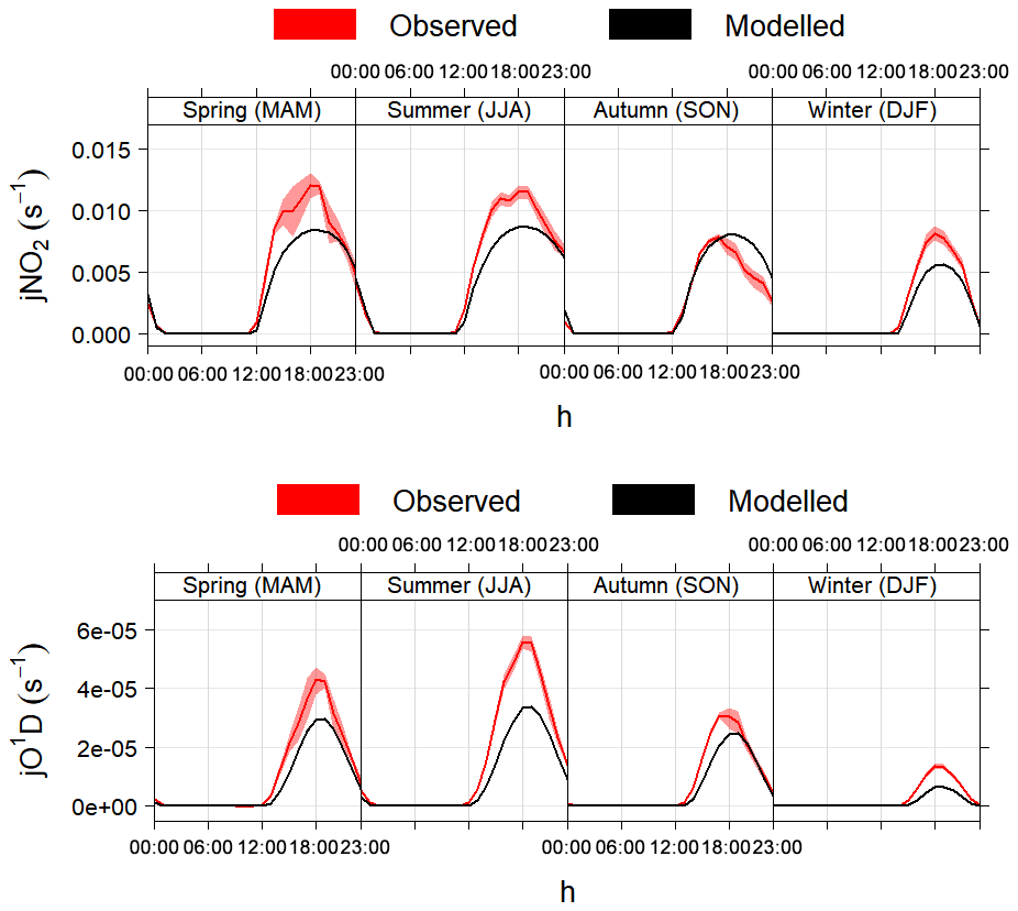
Figure 4Average modelled and measured j(NO₂) and j(O¹D) during different seasons in Boulder, CO, USA. The shaded areas are the 95 % confidence intervals of the mean. The timestamp is in Greenwich Mean Time, which is the timezone used by AtChem (local time is GMT−7 from November to February and GMT−6 from March to October).

Download

On average, the model underestimated the measurements of photolysis rates by 25 %–30 % in all seasons, with slightly better agreement (within 20 %) in autumn. The discrepancies between the modelled and measured values may be due to several factors: in particular, the two-stream isotropic scattering model used to derive the empirical parameters in the MCM is run for an altitude of 500 m and a latitude of 45^∘ N on 1 July (as described in Jenkin et al., 1997), while the measurements shown in Fig. 4 were taken at an altitude of ∼1700 m and a latitude of 40^∘ N in different seasons and years (between 2004 and 2009). Additionally, the model assumes clear-sky and ideal environmental conditions, which is often not the case during ambient measurements. The discrepancies between the model and the measurements thus highlight the importance of using measured photolysis rates (if available) and of using JFAC to correct the calculated photolysis rates, as explained above.

2.5 Model configuration

The typical workflow for AtChem2 is shown in Fig. 5: the user downloads the chemical mechanism from the MCM website, prepares the configuration files and chooses the model parameters. For AtChem-online a few extra steps are required, as the user has to upload the model configuration and data to the web server via the Web interface (Fig. 1). The configuration of AtChem sets the initial conditions, the list of constrained variables, the model start/stop date and time, the latitude and longitude, and the required model outputs. All the model configuration information and data are provided to AtChem in the form of simple text files, which can be prepared and edited with a normal text editor, thus simplifying the setup of the model and eliminating the need to modify the Fortran source code.

Figure 5Workflow of the AtChem2 model.

Download

Compilation of the AtChem model is done via a series of Python and shell scripts which link together the Fortran source code and the chemical mechanism – after conversion to a Fortran-compatible format, as explained in Sect. 2.2 – to create an executable file, called atchem (for AtChem-online) or atchem2 (for AtChem2). The compilation process is performed with a build script, which requires only a basic knowledge of the Unix command line: the user has to pass to the build script the path to the chemical mechanism file, the path to the configuration directory and the path to the model constraints. The model configuration and constraints are read by the executable at runtime: there is no need to compile the model more than once, unless the chemical mechanism or parts of the source code are modified by the user (Fig. 5). This approach makes it quick and easy to set up batch model runs. With AtChem-online batch model runs are not possible because compilation is automatically performed on the web server when the model run is started: the chemical mechanism, the configuration files and the model constraints have to be uploaded via the Web interface before every run and the model has to be recompiled every time it is executed, regardless of the changes that the user has made.

2.6 Integration and output

An atmospheric chemistry model is essentially a system of coupled ODEs that needs to be solved versus time for a given set of boundary conditions (Sect. 1). AtChem interpolates between the data points of the constrained variables, as explained in Sect. 2.3: the chemical species, the photolysis rates and the environment variables are evaluated by the solver when required and each is interpolated individually during the integration of the ODE system.

AtChem uses the CVODE library, which is part of the SUite of Nonlinear and DIfferential/ALgebraic equation Solvers (SUNDIALS; Hindmarsh et al., 2005) to integrate the system of differential equations; SUNDIALS is open source, under the BSD 3-Clause licence, and is available at https://computation.llnl.gov/projects/sundials/ (last access: 16 January 2020). Atmospheric chemical models are usually very stiff: this means they have at least one rapidly damped mode, corresponding to the short atmospheric lifetimes of some chemical species (of the order of seconds to minutes for the OH, HO₂ and RO₂ radicals) relative to the timescales of the full system (of the order of hours to months). The disparity in timescales results in the stiffness of the underlying ODE system. CVODE uses a multistep method with variable step-size and variable order to solve this type of stiff system. The solver type, preconditioner and other solver settings can be tuned by the user, although the default settings should be good enough for most atmospheric chemistry box models.

AtChem outputs the concentrations of the chemical species, the values of the environment variables, the reaction rates, the photolysis rates, and the model diagnostic variables. The Jacobian matrix can also be output, if required.

Reaction rates ($\mathtt{\text{k}}\times \left[\mathtt{\text{R1}}\right]\times \left[\mathtt{\text{R2}}\right]$, for the generic reaction $\mathtt{\text{R1}}+\mathtt{\text{R2}}\to \mathtt{\text{P1}}+\mathtt{\text{P2}}$) are output for all reactions in the chemical mechanism at a frequency chosen by the user in the model configuration. In addition, the model can calculate and output the rate of production and destruction for a selected number of species of particular interest. Rate of production/destruction analyses (ROPA/RODA) of short-lived reactive species are very useful to investigate the chemical budgets and fluxes of species of particular interest, such as the OH, HO₂, RO₂ and NO₃ radicals (Emmerson et al., 2007; Ren et al., 2008; Elshorbany et al., 2009; Sommariva et al., 2009; Lu et al., 2012). The ROPA/RODA model output consists of two formatted files with the rate of formation and loss of a given species for each reaction in which it is present as product or reactant, respectively. The species for which the calculated concentrations and the rate of production/destruction analysis are required are chosen by the user in the model configuration, together with the corresponding output frequency (Sect. 2.5).

All output files are simple space-delimited text files, which can be easily imported into external data analysis software for further processing and plotting. In AtChem2 the output files are saved in a directory specified by the user when the model run is started, while in AtChem-online the output files have to be downloaded from the web server as a compressed zip file. Simple plotting tools – in Python, R, MATLAB and gnuplot – allow the user to have a quick look at the model results and at the diagnostic variables as soon as the model run is completed.

3.1 Chamber studies

AtChem was originally conceived as a modelling tool for environmental chambers, in order to aid in the characterisation of the chambers, in the interpretation of the experimental results and in the evaluation/development of the MCM (Sect. 1). We demonstrate this type of application using data from a propene oxidation experiment conducted in the Chamber for Experimental Multiphase Atmospheric Simulation (CESAM), at the Laboratoire Inter-universitaire des Systèmes Atmosphériques, near Paris, France.

The propene chemical mechanism and the inorganic chemistry scheme were extracted from the MCM v3.3.1 and complemented with an auxiliary mechanism specific to the CESAM chamber, as described in Wang et al. (2011). Chamber-specific reactions are needed to model this type of experiment so that the background reactivity of the environmental chamber can be taken into account. This allows the separation of the chamber-specific chemical processes from the underlying processes that are being studied in the experiments, in order to make the results from experiments carried out in different chambers comparable and transferable to the atmosphere. The chamber-specific mechanism for CESAM includes chamber dilution, loss of O₃ and conversion of NO₂ to NO + HONO on the chamber wall, with an initial concentration of HONO of 8 ppbv (Wang et al., 2011). CESAM is an indoor atmospheric simulation chamber and uses three 4 kW xenon arc lamps as a light source. The photolysis rate of NO₂ was the only photolysis rate measured inside the chamber: during the propene oxidation experiment, when the chamber lamps were on, j(NO₂) was a constant value of $\mathrm{3.5}\times {\mathrm{10}}^{-\mathrm{3}}$ s⁻¹. The model was constrained to the j(NO₂) measurements, while the remaining photolysis rates were calculated by AtChem using the MCM parameterisation and scaled using the JFAC correction factor (Sect. 2.4).

Figure 6 shows the modelled mixing ratios of the precursor VOC (propene), with the primary oxidation products HCHO and CH₃CHO; the secondary product peroxyacetyl nitrate (PAN, formed via the OH + CH₃CHO reaction); and the inorganic species NO, NO₂, and O₃. The propene loss began when the chamber lamps were switched on – 1800 s after the start of the experiment – and was driven by reaction with OH, produced from HONO photolysis. HONO was formed in the chamber from heterogeneous chemistry occurring on the chamber wall; its role in initiating the oxidation of propene demonstrates that it is essential to understand, and include in the model, the chamber-specific chemical mechanism. The model showed good agreement with the observations of propene, NO, NO₂ and CH₃CHO, with a tendency to overestimate HCHO and underestimate O₃ and PAN in the latter stage of the experiment (Fig. 6), which may hint at potential problems with the chemistry of the oxidation products of propene in the MCM and/or with the chamber auxiliary mechanism. Such experiments can be used to refine and optimise the chamber-specific mechanisms, but, overall, the model results indicate that the MCM is reasonably accurate in its description of the gas-phase oxidation of propene in the troposphere.

Figure 6Measured (points) and modelled (lines) mixing ratios of propene (C₃H₆), ozone (O₃), nitrogen oxides (NO, NO₂) and propene oxidation products (HCHO, CH₃CHO, PAN) during a propene oxidation experiment at the CESAM atmospheric simulation chamber.

Download

3.2 Field studies

The chamber experiment and the corresponding model simulation shown in Sect. 3.1 are relatively simple: the chemical mechanism only had 83 species and 261 reactions, the model was unconstrained (except for j(NO₂)), and the duration of the experiment was less than 2 h. Intensive field campaigns typically last for several days or weeks and the chemical mechanism needed for a campaign model is usually much larger than the one needed for a chamber model. It is not unusual for a campaign model to use the entire MCM (>17 000 chemical reactions), along with a hundred or more constrained variables. This makes the model computationally very expensive and difficult to run on a web application, such as AtChem-online. AtChem2 was developed specifically for the long and complex simulations needed for field studies. We demonstrate this type of application using the dataset of the Texas Air Quality Study 2006, an intensive ship-based field campaign on the United States Gulf Coast (Parrish et al., 2009). The cruise took place between 27 July and 11 September 2006 on the NOAA research vessel Ronald H. Brown; the radical measurements (total peroxy radicals and NO₃) and the corresponding modelling study are discussed in Sommariva et al. (2011a). In that work, the model showed reasonably good agreement with the measured concentrations of total peroxy radicals (within ∼30 %, on average), although it underestimated the measurements of NO₃ by approximately a factor of 3.

The chemical mechanism used here was extracted from the MCM v3.1 (as in Sommariva et al., 2011a): it included the inorganic chemistry scheme, the oxidation mechanism of 65 VOCs, the dimethyl sulfide (DMS) oxidation mechanism from Sommariva et al. (2009), and dry deposition terms and heterogeneous reactions for the appropriate gas-phase species. The model constraints – CO, CH₄, H₂, NO, NO₂, O₃, SO₂, H₂O, 65 VOCs, j(O¹D), j(NO₂), j(NO₃), aerosol surface area, temperature, pressure, latitude and longitude – and configuration were the same as in the model described by Sommariva et al. (2011a).

The modelled concentrations of total peroxy radicals (HO₂ + RO₂) for the period 31 July–2 August are shown in Fig. 7, together with the corresponding measurements. The results obtained with version 1 of AtChem2 and with the beta version of AtChem used by Sommariva et al. (2011a) differ by ∼3 % – a discrepancy due to a small bug in the calculation of JFAC, which was fixed in a later version of AtChem. During the day, the model overestimated the measured concentrations of HO₂ + RO₂ by 10 %–25 %, which is well within the instrumental uncertainty (∼40 %). During the night, the model underestimated the measurements of HO₂ + RO₂ by up to 57 %, although the disagreement between the model and the measurements at nighttime during the entire cruise was on average lower (25 %–30 %; Sommariva et al., 2011a). The ability of the model to reproduce the observations of total peroxy radicals provides useful insight into the chemical processes in the marine boundary layer: the model-measurements discrepancies indicate that, under unpolluted conditions, radical chemistry is much better understood during the day than during the night, which suggests that future studies should focus on nocturnal chemistry.

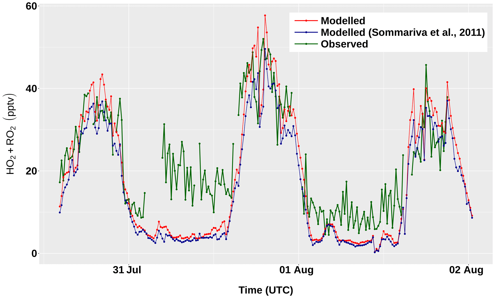
Figure 7Measured and modelled concentrations of total peroxy radicals (HO₂ + RO₂) between 31 July and 2 August, during the TexAQS 2006 cruise of the NOAA research vessel Ronald H. Brown.

Download

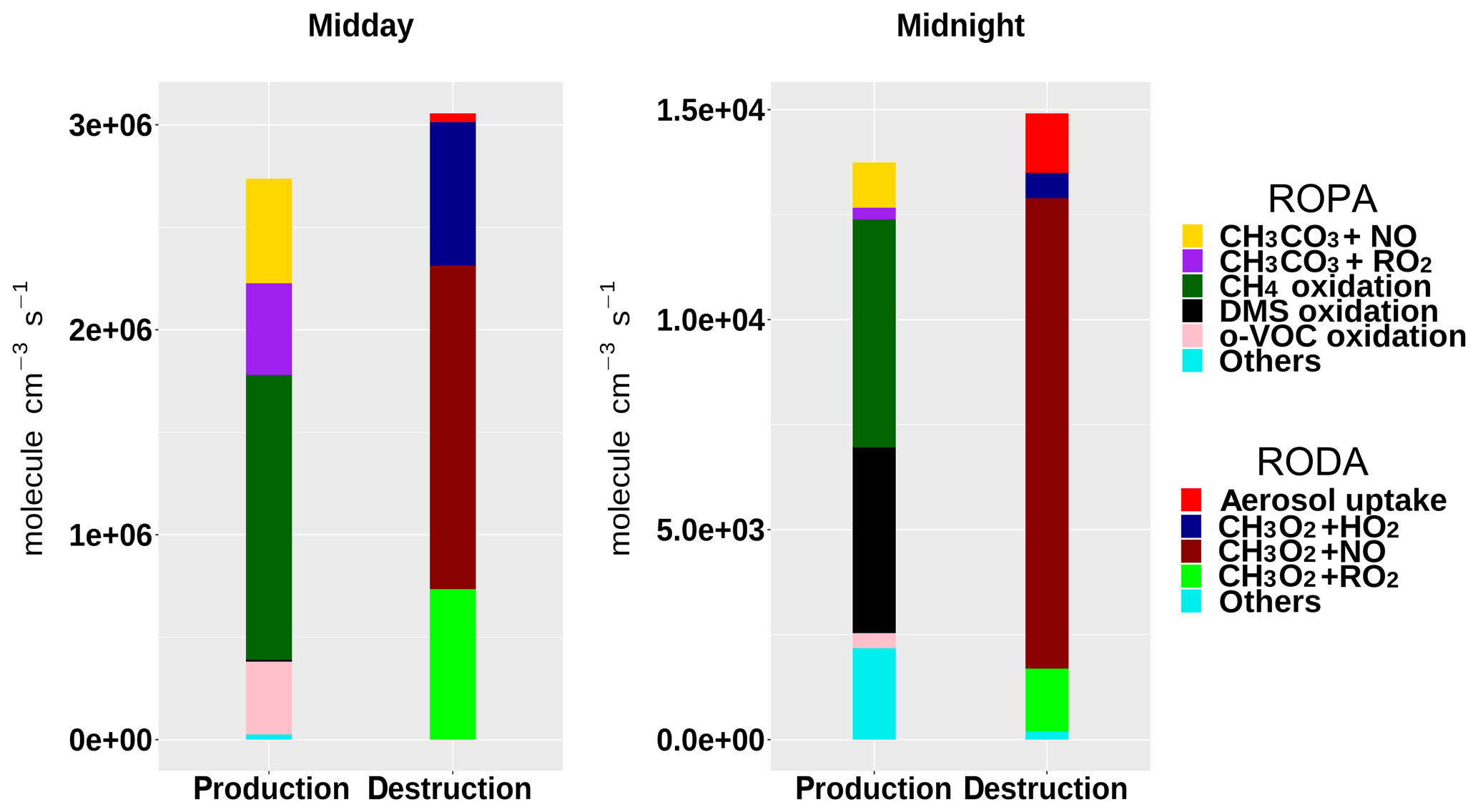
Figure 8Rate of production (ROPA) and destruction (RODA) analyses of the methyl peroxy radical (CH₃O₂) at midday and midnight of 1 August, during the TexAQS 2006 cruise of the NOAA research vessel Ronald H. Brown.

Download

The ROPA/RODA model output (Sect. 2.6) can be used to investigate the details of the chemical processes in the unpolluted marine atmosphere encountered during the first few days of TexAQS 2006. The model results indicate that, in that period, the methyl peroxy radical (CH₃O₂) was the major component of the RO₂ pool (30 %–45 % during the day, 50 %–80 % during the night). Figure 8 shows the rates of production and destruction of CH₃O₂ at midday and midnight of 1 August, when the ship was in the Atlantic Ocean off the coast of Florida. The main destruction term for CH₃O₂ was the reaction with NO, even though the levels of nitrogen oxides were low during the first few days of the cruise (<1 ppbv, on average). The reactions of CH₃O₂ with HO₂ and RO₂ accounted together for about half of the total CH₃O₂ loss at midday, but for only ∼15 % at midnight, because of the very low nocturnal concentrations of peroxy radicals. It must be noted, however, that since the model underestimated the concentrations of HO₂ and RO₂ during the night (Fig. 7), their role as CH₃O₂ sinks was also underestimated.

The oxidation of methane and the reactions of the acetyl peroxy radical – CH₃CO₃, typically formed from the oxidation of C₂–C₅ hydrocarbons – with NO and other peroxy radicals were the major sources of CH₃O₂. During the day, the oxidation of carbonyls and of organic acids was a significant contributor to the formation of CH₃O₂; at night, methane oxidation was driven by OH radicals formed by the ozonolysis of alkenes, while DMS oxidation (mostly via reaction with NO₃; Sommariva et al., 2011a) accounted for up to a third of the total CH₃O₂ production. The formation pathways of the methyl peroxy radical in the unpolluted marine atmosphere highlight the different chemical processes taking place during the day, when OH photochemistry dominates, and during the night, when reactions initiated by NO₃ and O₃ become an important source of short-chain organic peroxy radicals.