the Creative Commons Attribution 4.0 License.
the Creative Commons Attribution 4.0 License.
 | 06 Apr 2020
TIER version 1.0: an open-source Topographically InformEd Regression (TIER) model to estimate spatial meteorological fields
Martyn P. Clark
This paper introduces the Topographically InformEd Regression (TIER) model, which uses terrain attributes in a regression framework to distribute in situ observations of precipitation and temperature to a grid. The framework enables our understanding of complex atmospheric processes (e.g., orographic precipitation) to be encoded into a statistical model in an easy-to-understand manner. TIER is developed in a modular fashion with key model parameters exposed to the user. This enables the user community to easily explore the impacts of our methodological choices made to distribute sparse, irregularly spaced observations to a grid in a systematic fashion. The modular design allows incorporating new capabilities in TIER. Intermediate processing variables are also output to provide a more complete understanding of the algorithm and any algorithmic changes. The framework also provides uncertainty estimates. This paper presents a brief model evaluation and demonstrates that the TIER algorithm is functioning as expected. Several variations in model parameters and changes in the distributed variables are described. A key conclusion is that seemingly small changes in a model parameter result in large changes to the final distributed fields and their associated uncertainty estimates.


Gridded near-surface meteorological products (specifically precipitation and temperature) are a foundational product for many applications including weather and climate model validation, hydrologic modeling, climate model downscaling, among others (Day, 1985; Franklin, 1995; USBR, 2012; Pierce et al., 2014; Liu et al., 2017). It is often challenging to develop realistic estimates of these variables, particularly when complex terrain or large spatial climate gradients are present in the domain of interest. Because of their widespread usage and potential challenges generating products, a plethora of methods have been developed ranging from nearest neighbors, distance-weighted interpolation, Kriging, knowledge-based, climatologically aided interpolation, Gaussian filters, multiple linear regression, and others (Thiessen, 1911; Shepard, 1968, 1984; Chua and Bras, 1982; Daly et al., 1994; Willmott and Roebson, 1995; Thornton et al., 1997; Banerjee et al., 2003; Clark and Slater, 2006; Cressie and Wikle, 2011; Nychka et al., 2015; Cornes et al., 2018).
Across the methods, nearest neighbor and distance-weighted interpolations use spatial distance as the only predictor, a reasonable choice in areas with high station densities but much less so in sparsely gauged regions. The resultant field is also discontinuous between station areas of influence for nearest neighbor, while distance-weighted interpolation will increase precipitation occurrence unless explicit occurrence prediction is included (Thornton et al., 1997; Newman et al., 2015, 2019). Climatologically aided interpolation assumes the climatological field is better resolved by the available observations and has a strong relationship with the field of interest (e.g., daily precipitation) such that using the climatological field in the final interpolation increases the output information content (Willmot and Robeson, 1995). These assumptions are invalid when the climatological field is poorly resolved, or has little correspondence to the field of interest which happens when an event has a significantly different pattern than climatology (e.g., Lundquist et al., 2015; Newman et al., 2019). Kriging and linear regression frameworks may include multiple spatial predictors and uncertainty estimates. However, these methods may also produce unrealistic results with sparse station observations (Cornes et al., 2018). Finally, knowledge-based systems impose a regularization on the input data through knowledge-based rules (Sect. 2). This allows for physically plausible interpolation fields in sparsely gauged regions but inflexibility similar to climatologically aided interpolation. Finally, in sparsely observed regions, we do not know the true error characteristics of any method.
The currently available climate products that use these methods have complex processing systems (Daly et al., 2008; Xia et al., 2012; Livneh et al., 2015; Newman et al., 2015; Thornton et al., 2018). The product workflow typically includes many processing steps, methodological choices, and model parameters, all interacting to influence the characteristics of the final product. Therefore, comparison studies of product performance (and even single product evaluations) are often not able to attribute differences at the final output level to specific methodological choices (Newman et al., 2019). To help alleviate these difficulties and improve our understanding of method performance across conditions, flexible modular software systems need to be developed that expose model parameters to the users and allow for new functionality to be easily added (Clark et al., 2011).
This paper focuses on approaches that incorporate knowledge of atmospheric physics into relatively simple underlying statistical models (e.g., orographic precipitation, temperature lapse rates into linear regression models) to improve the accuracy of the gridded field (e.g., Daly et al., 1994; Willmott and Matsuura, 1995). Daly et al. (1994), hereafter D94, develop a complex knowledge-based system consisting of (1) terrain pre-processing; (2) station selection; (3) development of a locally weighted meteorological variable-elevation linear regression; and (4) post-processing. Omitted here are the pre-processing steps to screen station data (including quality control) and filling missing or suspicious data values. Following D94, many studies have included new knowledge-based capabilities, new intermediate processing steps, and increased granularity in a given step (Daly et al., 2002, 2007, 2008). In recent papers, there are upwards of 15–20 model parameters that have varying degrees of influence on the final product.
The Topographically InformEd Regression (TIER) model implements the knowledge-based approach described in D94 and subsequent papers (Daly et al., 2000, 2002, 2007, 2008; hereafter D00, D02, D07, and D08). Note that TIER is not designed to be an exact replica, as it does not match any source code, nor does it implement all features described in D94, D00, D02, D07, and D08. The paper is organized as follows: we introduce the TIER conceptual model in Sect. 2.1, the pre-processing algorithms in Sect. 2.2, the regression model in Sect. 2.3, and post-processing routines in Sect. 2.4. Then, a brief model evaluation is included in Sect. 3 to verify that the TIER model is functioning as expected. Next, we explore model parameter variation experiments for three simple test cases to highlight how model parameter choices impact the final product in Sect. 3.1. Finally, a summary discussion of TIER, lessons learned from the parameter experiments, and next steps are discussed in Sect. 4, with code and data availability provided at the end of the paper, respectively.
2.1 Conceptual model
Precipitation and temperature are unevenly distributed around the globe for myriad reasons including general circulation patterns and landscape effects. Following D94, TIER assumes that large-scale gradients are resolved by the input station data and incorporates direct knowledge of atmospheric physics to account for landscape effects (e.g., orographic precipitation, mesoscale circulations near the coast). Since the landscape influences the distribution of precipitation and temperature, particularly their climatology, many past studies have developed methods to use terrain attributes to estimate meteorological fields (e.g., Spreen, 1947; Phillips et al., 1992). For example, orography has a particularly strong influence on precipitation by enhancing uplift of air (e.g., Schermerhorn, 1967; Smith and Barstad, 2004).
D94 develops a method to use a high-resolution digital elevation model (DEM) to produce empirical estimates of the precipitation–elevation relationship. They demonstrate that using actual station elevations in the precipitation–elevation relationship leads to a weak or nonexistent relationship, while using a coarse-resolution DEM smooths out local variability and results in a stronger relationship between precipitation and elevation. Such stronger relationships occur because microscale terrain features have a much smaller impact on the atmosphere than the larger-scale terrain features of the order of 2–15 km (D94 and references therein). Of course, the optimal length scale varies across atmospheric conditions and for each precipitation event, but in general a coarse-resolution or smoothed high-resolution DEM provides a strong basis for developing robust climatological precipitation–elevation relationships. Additionally, the amount of precipitation varies according to aspect (e.g., windward or lee slope), suggesting the need for different relationships for different aspects (e.g., Alter, 1919; Houghton, 1979). D94 use the smoothed DEM and decompose the domain into directional “facets” that all individually have a separate precipitation–elevation relationship. Facets are defined as continuous areas with similar aspects (slope orientation).
Daly and his colleagues have introduced several methodological enhancements since the seminal D94 paper. D00 expand on D94 to include maximum and minimum temperature, while D02 fully describe the knowledge-based system and the various physical processes included in it. Beyond elevation, the influence of large bodies of water on precipitation and temperature are incorporated by using coastal proximity or distance to the coastline. Finally, cold-air drainage down slopes and subsequent pooling in valleys is modeled as well. A conceptual two-layer atmosphere where layer 1 is the boundary layer containing temperature inversions and layer 2 is the free atmosphere is applied to the DEM. A simple two-layer atmospheric model for temperature is necessary to capture near-surface temperature inversions. This method identifies areas highly susceptible to inversions (e.g., valleys) and allows for the model to have temperature lapse rate reversals from increasing temperature with height below to decreasing above the inversion. Grid points that are identified to be within the boundary layer (layer 1) are allowed to have strong temperature inversions. These grid points are identified using the topographic position concept, which essentially computes the average nearby topographic relief to identify valleys and ridges. D94, D02, and D08 provide extensive details on the underlying theory of this knowledge-based approach.
2.2 TIER terrain pre-processing
The TIER pre-processing routines consist of the functions used to generate the required terrain attributes for the regression model. Currently, this consists of functions that perform NetCDF input/output (IO), process the DEM into topographic facets, the distance to the coast, topographic position, and estimate the idealized two-layer atmosphere. A parameter and control file specifies model parameters, and IO directories and files; see Tables 1 and 2, respectively. A flowchart describing the general flow, order of operations, and data requirements is given in Fig. 1.
Table 1Terrain pre-processing model parameters.
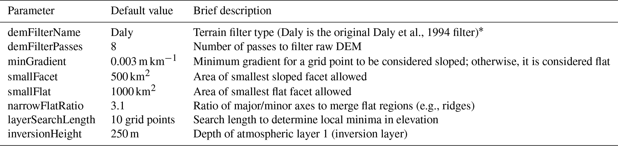
* Only filter option currently implemented.
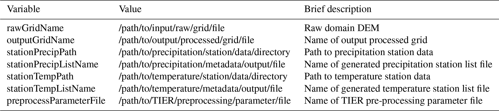
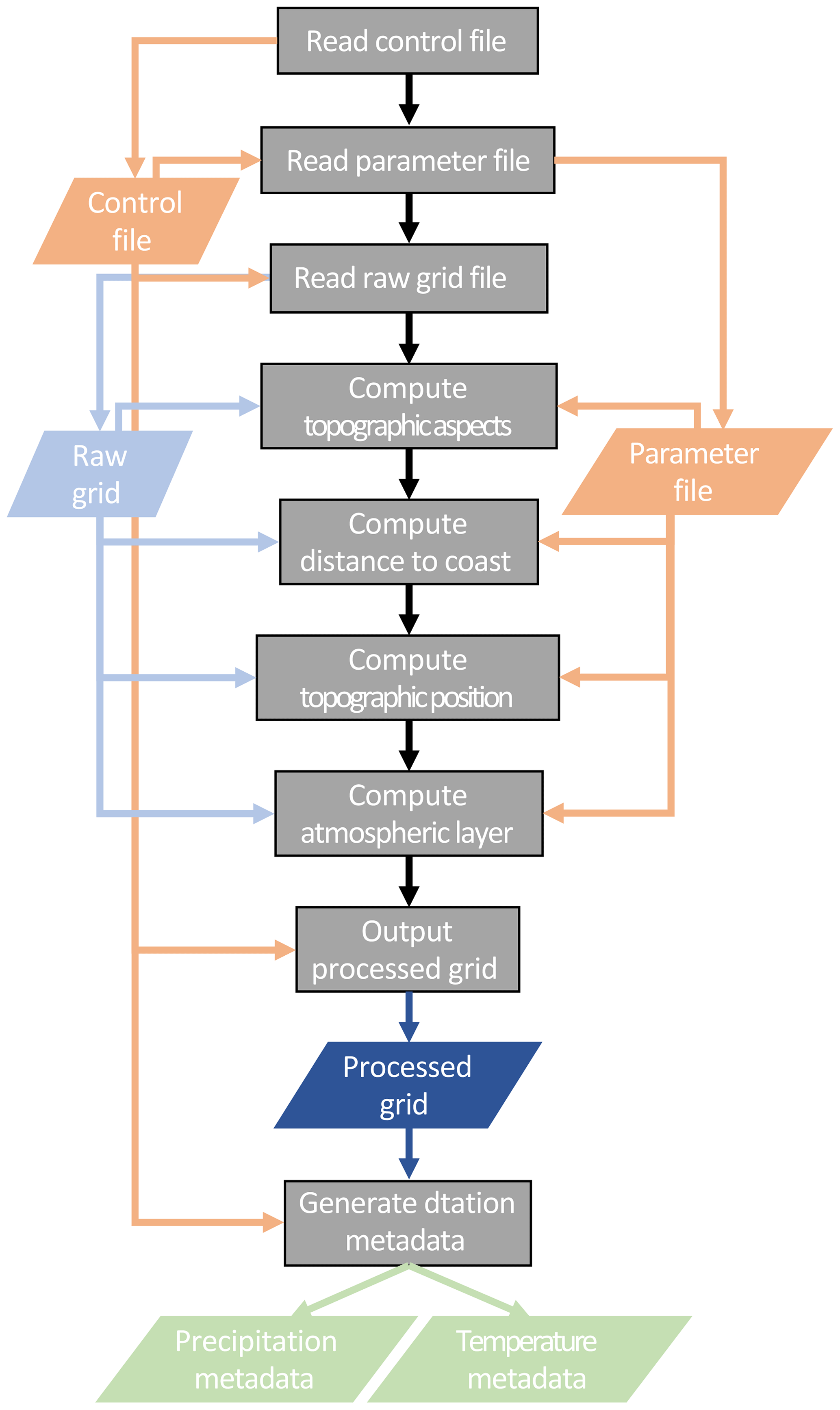
Figure 1Flowchart describing the TIER pre-processing system. Processes are shaded gray, input files are orange, topographic inputs and outputs are shades of blue, and outputs are various shades of green.
2.2.1 Topographic facets
The native resolution DEM is first smoothed using a user-defined filter (Table 2). The “Daly” filter is defined as (D94)
where is the smoothed elevation and Ei,j is the high-resolution elevation at grid point (i, j). D94 computes multiple smoothed DEMs to account for data density changes across the domain, while TIERv1.0 only computes one smoothed DEM. Once the smoothed DEM is calculated, the slope aspect (0–360∘) is computed and facets are defined. There are five (5) facets in TIERv1.0: (1) north (aspect >315∘, aspect ); (2) east ( aspect ); (3) south ( aspect ); (4) west ( aspect ); and (5) flat (D94). Flat aspects are areas with terrain gradients (slopes) less than the user-specified minGradient (m km−1, Table 2). After the facets are defined, small facets are merged together with neighboring facets using the minimum size model parameters (Table 2). Flat regions that are very narrow are considered ridges and behave like neighboring facets. These are merged into the neighboring facets on the west or south slopes depending on their orientation (D94).
2.2.2 Distance to the coast
The user defines a land–ocean mask field in the input grid file. This mask defines which grid points are large bodies of water (ocean points) and are used in the coastal proximity calculation. The distance to the coast is computed using the great circle distance assuming a spherical earth for every grid cell within a user-defined distance threshold.
2.2.3 Topographic position
To identify the atmospheric layer (Sect. 2.2.4) of a grid point, the local topographic position of a grid point is computed first. The topographic position calculation uses the high-resolution DEM. Following D02, for each grid point, the following steps are taken.
The minimum elevation within a user-defined local search radius (r, Table 2) is found. D02 suggest a search radius of 40 km.
where denotes the DEM elevations within ±r grid points at valid land points in the i and j directions, and is the local minimum elevation.
The topographic position is then estimated as
where Ng is the number of land grid points within the search radius (Ng≤r2).
2.2.4 Two-layer atmosphere
Following the determination of the topographic position, each grid cell is placed into the first (boundary or inversion layer) or second layer (free atmosphere) of the idealized two-layer atmosphere. The height of the inversion layer is defined by the user (Table 2) and added to the mean elevation computed on the left-hand side of Eq. (3). This defines an inversion height above sea level for all grid points. All grid points where Ei,j is less than the inversion height are placed into layer 1, while all other grid points are placed into layer 2 (D02).
2.2.5 Station metadata
After the input domain grid file has been processed, the pre-processing routine generates station metadata files for all precipitation and temperature stations that will be used in the regression model. Each station is assigned the closest grid point value of the smoothed DEM, facet, topographic position, atmospheric layer, and coastal distance.
2.3 Interpolation model
The regression model is applied to each land-masked grid cell. It consists of routines to compute the station weights, to estimate the meteorological–terrain relationships, and to estimate the variable value at each grid point. A parameter and control file specifies model parameters, and IO directories and files; see Tables 3 and 4, respectively. A flowchart describing the general flow, order of operations, and data requirements is given in Fig. 2. Figures 3 and 4 provide more detailed flowcharts for the specific processing flow for precipitation and temperature variables.
Table 3TIER model parameters. Default values are given for precipitation with values for temperature given in parentheses.
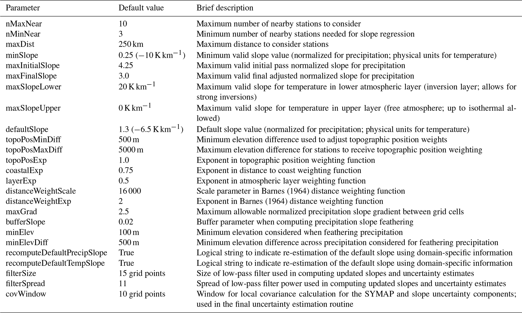


Figure 2Flowchart describing the TIER processing algorithm including post-processing. Color shading is the same as that in Fig. 1.
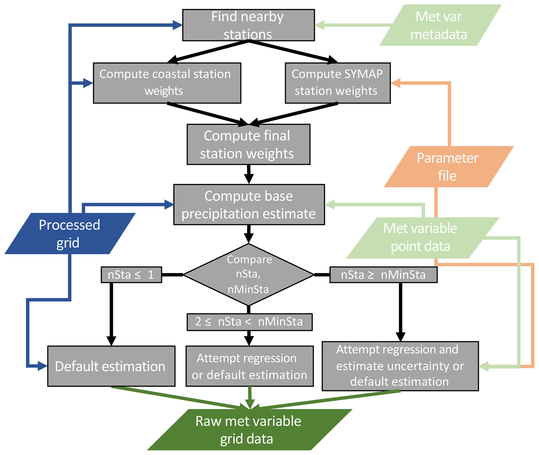
Figure 3Flowchart describing the precipitation grid point estimate algorithm. Color shading is the same as that in Fig. 1.
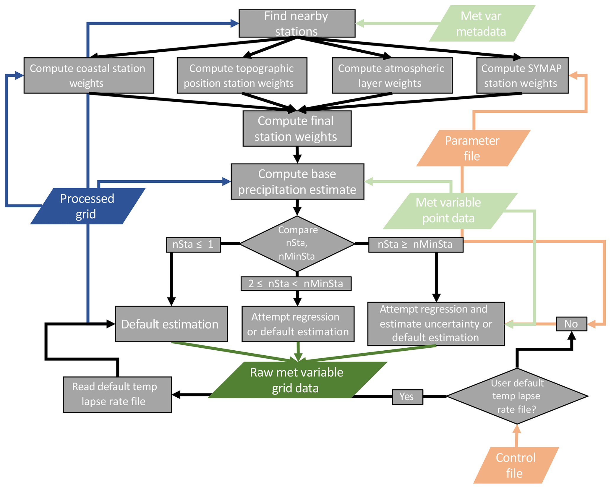
Figure 4Flowchart describing the temperature grid point estimate algorithm. Color shading is the same as that in Fig. 1.
2.3.1 Station selection and weighting
For each grid point, a set of stations is used to estimate the precipitation and temperature values. First, all stations within the user-defined search radius are found (nearby stations), up to the maximum number of stations considered (Table 4). From that subset of stations, all stations on the same facet as the current grid point are identified (facet stations). Then, a set of distance-dependent weights and weights for each physical process component described in Sect. 2.2.1–2.2.4 is generated for all nearby and facet stations for each grid point. These component weights are then combined to create the final station weight vector.
where W is the final weight vector, Wd is the distance-dependent weights, Wf is the facet weights, Wl is the atmospheric layer weights, Wt is the topographic position weights, and Wp is the coastal proximity weights. All component weights and the final weight vector are normalized to sum to unity (D02). For precipitation, only Wd, Wf, and Wp are used to estimate W, while temperature uses all five component weights in W.
Distance-dependent weighting
A station's relevance to the current grid point decreases as the station distance increases (e.g., Shepard, 1968); thus, this component station weighting decreases with increasing distance. Here, we generally follow the synagraphic computer mapping (SYMAP) algorithm of Shepard (1968, 1984) and develop inverse distance weights that are further modified by including direction information. Direction information is used to downweigh stations that are in a similar direction but further distance than other stations, as their influence has been “shadowed” by the nearer station (Shepard, 1968). The distance weighting function of Barnes (1964) is used:
where I is the inverse distance-dependent weights, d is the station distance vector, and y and s are the user-defined Barnes exponent and scale factor, respectively (Table 4). The angle-dependent weights are then computed as (Shepard, 1984)
where Ts is the station angle weight for station s, and subscripts s and q denote station subscripts for stations 1:nx, where nx is the maximum number of stations considered for each grid point (Table 4). The final distance-dependent weights are then computed as
where n is the number of stations considered at the current grid point. Wd is then normalized to sum to unity.
Facet weighting
Stations on the same facet type as the current grid point receive an initial facet weight of 1. D02 introduces a method to reduce the weight of stations on the same facet type but with intervening facets of different types between the station and grid point (D02 Eq. 5). This is not implemented here, and all stations on the same facet type as the current grid point receive the same weight. This could be a decision considered for exploration in a future TIER release. The distance-dependent weights already account for this implicitly, but the explicit inclusion of additional weight decreases for stations on the same facet type will increase the localization of the TIER station weighting even further. This would increase the small-scale features of TIER.
Atmospheric layer
The atmospheric layer weight function is defined as
where Δls is the layer difference between the grid point and station s, the elevations are defined using the high-resolution DEM and station elevation (Es), and a is the user-defined layer weighting exponent (Table 4). Following D02, stations in the same atmospheric layer as the current grid point receive an initial weight of 1. D02 includes an additional check to see if the station–grid elevation difference is smaller than some threshold value for a station. If this is true, a station in a different layer and grid cell may still receive a weight of 1. TIERv1.0 does not include the additional conditional statement and only stations in the same atmospheric layer receive an initial weight of 1. The vertical elevation difference is then used to weigh the remaining stations. The atmospheric layer weighting is applied only to temperature variables in TIERv1.0.
Topographic position
The topographic position weights are computed following D07:
where Δts is the topographic position difference between the current grid cell and station s, Δtm and Δtx are the user-defined minimum and maximum topographic position differences, and z is the topographic position weighting exponent (Table 4). The topographic position weight enhances identification of stations that lie in similar topographic areas (e.g., valleys) and is applied only to temperature variables in TIERv1.0.
Coastal proximity
Using the computed distance to the coast, the coastal proximity weights are computed as
where Δps is the absolute difference between the current grid cell and station s distance to the coast values, and c is the user-defined coastal proximity weighting exponent (Table 4). D02 computes coastal proximity weights using the same inverse distance function but also includes a threshold (Δpx), which, if Δps>Δpx, is set to zero. This weighting factor highlights stations with similar coastal proximity to the current grid cell.
2.3.2 Grid point estimate
Once nearby stations are selected and the final weight vector is computed (Eq. 4), a base grid point estimate is developed using the weighted average of all nearby stations:
where is the grid point meteorological variable estimate, and Ys and Ws are the observed station value and the station weight for station s, respectively. The uncertainty of this value is estimated as the standard deviation of the leave-one-out estimates, which is all possible combinations of nr−1 stations, , which in this case are nr possible combinations.
where nr is the subset of stations that are both within the distance threshold and on the same facet as the current grid cell, is the estimated standard deviation of , and is the estimated value when the ith station is withheld.
Next, the variable-elevation linear regression coefficients are solved for
where β is the vector of linear regression coefficients (βo,β1), As is the nr×2 design matrix, W is the nr×nr diagonal weight matrix populated with the final weight vector W, and Y is the vector of observed station values. In D94, D02, and D08, these coefficients determine the grid point estimate as
where β1M and β1X are the user-defined minimum and maximum valid regression slopes (Table 4). Note that slope here is in physical units per distance (e.g., mm km−1 or K km−1), which is also referred to as the lapse rate in atmospheric science. In TIERv1.0, we have chosen to use the base grid point estimate, , as the intercept value in the variable-elevation regression equation. This is done because when falls outside of the bounds in Eq. (14), a default slope value is used, but is not modified. Thus, the base estimate of a variable for a grid cell is sometimes derived from an equation the system considers invalid. Therefore, we fully disassociate the intercept and slope estimates. Here, we provide an initial assessment of this choice in Sect. 3, but this methodological choice should be examined in more detail in future work. Subsequently, we then also modify the elevation used in the regression equation to be the difference between the high-resolution DEM elevation and the W weighted station elevation using the smoothed DEM station elevations. The switch to an elevation difference is required as we are effectively correcting the base estimate to the DEM elevation, and the base estimate has an intrinsic elevation associated with it. Therefore, the TIERv1.0 grid point estimate is
where ΔE is the difference between the smoothed DEM elevation and the W weighted station elevation using the smoothed DEM station elevations. When is invalid, the default slope is used, and when the initial is valid, the uncertainty of is estimated in a similar manner to that of using Eq. (12). Note that for temperature variables only, the user can define a spatially variable default lapse rate (Table 3, Fig. 4). The standard deviation of all valid slope estimates from the leave-one-out estimates, , is used as the uncertainty estimate of :
where is the estimated standard deviation of and is the estimated value when the ith station is withheld.
D02 define the method to adaptively adjust the station search radius until the minimum number of needed stations is met. Here, we do not adjust the search radius and instead attempt the regression and uncertainty estimation when nr≥nm, where nm is the user-specified minimum number of stations required for the regression (Table 4). When nr<nm, the regression is attempted for , and the default slope is used when nr<2. Additionally, for nr<nm, Eq. (16) is never applied and there is no direct uncertainty estimate of for those grid cells.
Finally, D94 found that normalizing the precipitation lapse rate (km−1) after performing the regression reduces the large spatial variability in precipitation lapse rates due to the large spatial variability in the underlying precipitation amounts. The normalization is done at each grid cell as
where
where is the mean precipitation (mm) of all stations considered for the regression for the current grid point, is the estimated slope in physical units (mm km−1), and YP,s is the station precipitation (mm) at station s. Accordingly, is
The normalization allows for the bounds in Eqs. (14)–(15) to be broadly applicable for precipitation, as well as for a reasonable default lapse rate to be applied to grid points where a valid regression slope cannot be found. Temperature lapse rates are computed in physical units (K km−1), as there is little variability in temperature lapse rates.
2.4 Post-processing
Several post-processing steps are undertaken to reach the final gridded estimates after all grid points have an initial estimate, shown in Fig. 5. These include updating estimated slope values, applying spatial filters, and recomputing the final fields.
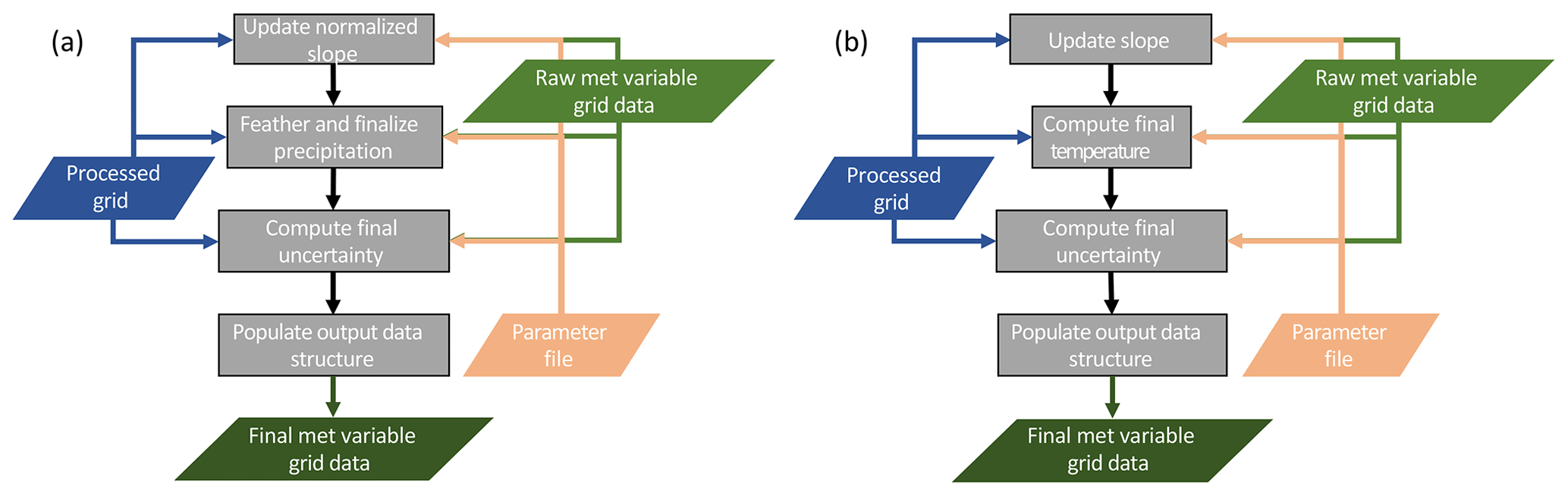
Figure 5Flowcharts describing the (a) precipitation post-processing and (b) temperature post-processing. Color shading is the same as that in Fig. 1.
2.4.1 Precipitation
The initial precipitation normalized slope estimates are used to recompute the default slope if the user specifies (Table 4). In this case, all grid points with valid regression slopes are used to compute the domain mean normalized precipitation slope. This value is then substituted at all grid points with default slope estimates. Next, a 2-D Gaussian filter is applied to the normalized slopes to reduce noise and smooth the artificial numerical boundaries in slope values and is taken as the final precipitation slope estimate (Fig. 5a). The parameters of this spatial filter (size and spread) are specified in the TIER model parameter file (Table 4).
After the slope estimates have been finalized, the precipitation is field is recomputed using Eq. (15) and then a feathering process is applied to smooth any remaining very large gradients (e.g., D94; Fig. 5a). The feathering routine operates on the normalized precipitation slopes and searches for grid cell–grid cell gradients in the normalized slope larger than a user-specified value (Table 4). If a large gradient is found, the slope of the grid cell with less precipitation is increased until the gradient falls below the maximum allowable value. The feathering routine iterates over the grid until there are no remaining large gradients and is an additional smoothing step for precipitation in TIER. Also, the feathering routine only runs for grid cells with larger elevation changes than a user-specified minimum gradient (Table 4), which effectively ignores flat areas (D94), and in TIERv1.0 the feathering routine only operates on grid cells above a user-specified minimum elevation.
Finally, uncertainty estimates are recomputed for the entire grid, first for the base estimate and slope components, then for the total uncertainty of Eq. (15) (Fig. 5a). For those grid points with no initial , the nearest neighbor estimate is used. Then the same Gaussian filter applied to the normalized precipitation slopes is applied to the gridded and . The final uncertainty contribution due to uncertainty in the precipitation slope at a grid point in physical units (mm) is then computed as
where is the final uncertainty (mm) due to uncertainty in the precipitation slope, is the final slope uncertainty (mm km−1), and is the final precipitation estimate (mm). The filtered field is used as the final base precipitation estimate, . The total uncertainty is estimated as the combined standard deviation of the two component estimates:
because the covariance between the two component uncertainties is sometimes nonzero. The covariance is computed locally at each grid point using a user-defined 2-D window of points (Table 4) around the current grid point.
2.4.2 Temperature
Post-processing for temperature is simpler than that for precipitation because the temperature lapse rates are in physical units. The initial valid temperature slope estimates are used to recompute the default lapse rate if the user specifies (Table 4) when there is no spatially varying default temperature lapse rate information provided (Table 3). Again, the mean of all valid regression slope estimates is used as the updated default temperature lapse rate for this case. As for precipitation, a 2-D Gaussian filter is then applied to the slopes to reduce noise and smooth the artificial numerical boundaries in slope values and is taken as the final temperature slope estimate (Fig. 5b). Then, the final temperature estimate is computed using these updated lapse rate values and Eq. (15).
As for precipitation, the component and total uncertainty estimates are then finalized for temperature. The base temperature estimate uncertainty and slope uncertainty are smoothed using the 2-D Gaussian filter to estimate the final component uncertainties, and , respectively. Then, the final temperature uncertainty contribution due to temperature lapse rate uncertainty is computed using Eq. (18), and Eq. (19) is used to compute the total uncertainty of the temperature estimate, substituting subscript Ts for Ps in both.
An example use case over the western United States, focused primarily on the Sierra Nevada mountains between roughly 35–43∘ N and 118–125∘ W including precipitation, maximum (Tmax) and minimum (Tmin) temperature data (Fig. 6), is used for computing basic model evaluation statistics. This evaluation is to simultaneously determine if the TIERv1.0 algorithm is performing as expected numerically and to provide a brief baseline of performance. We calculate bias and mean absolute error (MAE) statistics from the final gridded meteorological variables using all available stations or a calibration sample evaluation. Additional evaluation is considered outside the scope of this initial presentation of the model.
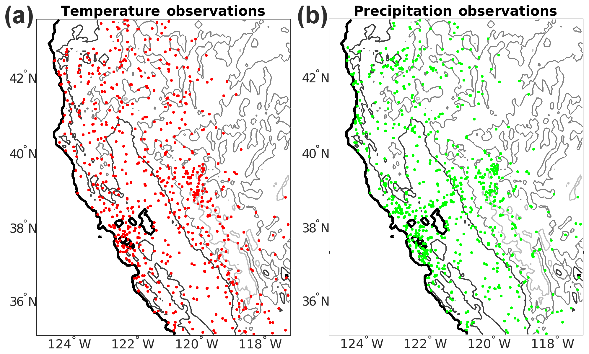
Figure 6The TIER test domain with (a) the temperature station distribution and (b) the precipitation station distribution. Contours indicate the 0, 500, 1500, and 2500 m elevation contours moving from black to light gray.
The gridded output fields are nearly unbiased for all three variables: 0.2 mm, −0.22, and −0.21 K for precipitation, Tmax, and Tmin, respectively. MAE values are 0.84 K for Tmax and 0.75 K for Tmin and 14.3 mm for precipitation (Table 5). Additionally, the gridded output values have nearly zero conditional bias for temperature, as indicated in Fig. 7a–b, where the fitted slope to the TIER–observation points is 0.93 and 0.96 for Tmax and Tmin, respectively. There is an overestimation at smaller values transitioning to an underestimation at larger values. Precipitation has the same conditional bias structure as temperature (Fig. 7c); however, the slope of the TIER–observation fitted linear regression is 0.88, indicating a larger conditional bias as observed precipitation increases.
Table 5Calibration sample evaluation statistics for TIER using the default parameters with 90 % confidence intervals in parentheses.
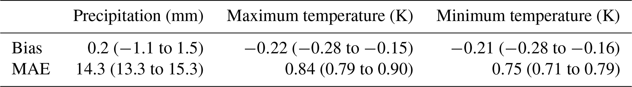
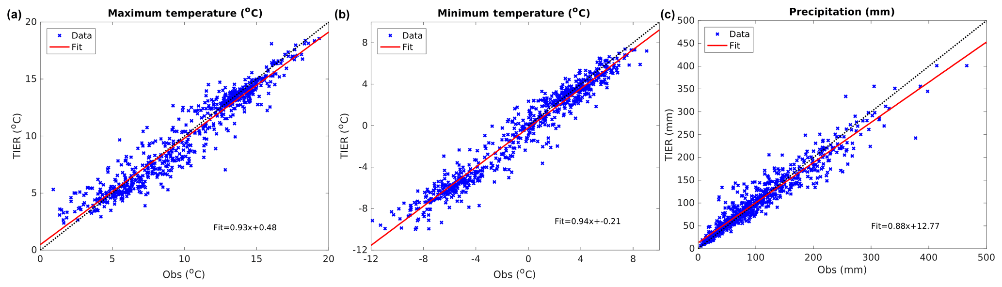
Figure 7Calibration sample evaluation scatter plots (TIER versus observations) for (a) maximum temperature (∘C), (b) minimum temperature (∘C), and (c) precipitation (mm).
Figure 8 highlights the methodological choice made in Sect. 2.3.2 to disassociate the intercept parameter from the regression estimated slope in Eq. (15) for precipitation. We compare estimates using (PRISM-similar) in Eq. (15) versus (TIERv1.0) and find that in general precipitation estimates using are larger than those of TIERv1.0, particularly at higher elevations. TIERv1.0 has mean precipitation for grid points below and above 2000 m of 83.2 and 88.6 mm, respectively. The PRISM-similar method has average precipitation values of 117.6 and 152.3 mm above and below 2000 m, which are 42 % and 72 % increases over TIERv1.0. Comparison to in-sample station observations shows that the estimation method results in higher biases and MAE than TIERv1.0: 38.2 versus 0.2 mm bias and 51.9 versus 14.3 mm MAE for the two methods, respectively.

Figure 8Comparison of precipitation (mm) estimates using in Eq. (15) versus TIERv1.0 which uses in Eq. (15).
These differences could be due to several reasons, including that TIERv1.0 parameters were subjectively tuned for the published methodology. Also, in-sample validation does not truly determine method performance, an out of sample verification exercise and further evaluations should be undertaken. The PRISM-similar method within the PRISM model performs extremely well and may likely be more appropriate for higher elevations given the tendency for these types of linear regression systems to underestimate precipitation above the highest observation when using smoothed DEM values (see Sect. 4d.4 and parameter B1EX in Table 1 of D94).
3.1 Model parameter experiments
Here, we explore the impact of model parameter changes on the output values and their associated uncertainty estimates. We modify TIER model parameters only (no pre-processing parameters) and make three parameter changes to parameters focused on different parts of the interpolation model for different variables in an effort to concisely highlight how model parameter choices impact the final product. First, we modify the inverse distance weighting exponent in the distance-dependent weighting function for Tmin (experiment 1), then we modify the coastal distance weighting exponent for precipitation (experiment 2), and finally we modify the maximum number of stations allowed for each grid point for precipitation (experiment 3).
Table 6Calibration sample evaluation statistics for the three experiments.

3.1.1 Experiment 1
In experiment 1, the parameter “distanceWeightExp” (Table 4), which is the exponent in the distance-dependent weighting function (Eq. 5), is modified from 2 (default) to 1.75 (modified) for a spatial simulation of Tmin. This decreases the negative slope of the inverse distance weighting function such that stations further from the considered grid point receive more weight in the modified case than the default. The resulting Tmin distributions and difference field are given in Fig. 9. The spatial distributions are very similar throughout most of the domain as the observation network is relatively high density across most of the domain (Fig. 6). Where the station density decreases along the eastern side of the domain, differences increase in magnitude east of 119∘ W. Notably, there are also pockets of differences outside of ±1 ∘C in areas with high station density along the coast and between 40–42∘ N and 121–123∘ W. These locations contain complex terrain, specifically large elevation gradients, and the modified station weights result in different estimated temperature lapse rates in addition to changes in the base estimate, resulting in the different temperature estimates. However, the calibration sample statistics are not significantly different at the 90 % confidence level than the default parameter set (Table 6), suggesting that the changes in the gridded field are not able to be differentiated in a meaningful way.

Figure 9Spatial distribution of minimum temperature (Tmin, ∘C) for model parameter sensitivity experiment 1. (a) Default model parameters, (b) modified distance weighting exponent, and (c) the difference field (default – modified).
3.1.2 Experiment 2
For experiment 2, we examine precipitation and modify the “coastalExp” (Table 4) parameter from 0.75 to 1 to examine the influence of changes to the coastal proximity weighting. Qualitatively, the two precipitation distributions are identical to the overall precipitation pattern, remaining essentially unchanged (Fig. 10a–b). The difference fields show that there are shifts in the precipitation placement throughout the domain through the alternating positive/negative difference patterns, particularly across the complex terrain (Fig. 10b), but essentially there is no net precipitation change with a total relative difference of 0.2 % between the two estimates. Absolute differences can be as large as 46 mm in areas of large total accumulations; however, the relative differences in those areas are generally less than 10 % (Fig. 10b). Correspondingly, dry areas have smaller absolute differences but sometimes larger relative differences, as can be seen along the eastern third of the domain (Fig. 10b). The mean absolute value of the cell-to-cell precipitation gradient is 1.56 mm km−1 versus 1.69 mm km−1 (8.3 % increase) in the base and modified cases, respectively. Increased station localization should be expected to increase high-frequency variability and thus spatial gradients. The calibration sample statistics are not significantly different at the 90 % confidence level from the default parameter set (Table 6). However, in this case, the confidence bounds are almost all non-overlapping, which may suggest increasing the coastal exponent further would improve the model performance.

Figure 10Spatial distribution of (a) base precipitation (mm) for model parameter sensitivity experiment 2, (b) default – modified precipitation difference (mm), and (c) default – modified uncertainty difference (%).
The total uncertainty is generally increased by a few millimeters across the domain (0.55 mm on average), with a corresponding relative increase in uncertainty of around 5 %–10 % (Fig. 10c). This is due to the fact that increasing this weight exponent decreases the weight of stations more dissimilar to the current grid point, effectively increasing the localization of the weights and increasing the variability of the leave-one-out estimates (Eq. 16).
3.1.3 Experiment 3
Finally, we change the “nMaxNear” parameter (Table 4) from 10 to 13, which controls the maximum number of stations used for each grid point the interpolation model. Again, the precipitation pattern is essentially qualitatively unchanged between the two configurations with a 0.2 % domain average change; also see Fig. 11a. However, the relative difference fields highlight larger and more systematic changes to the precipitation distribution than in experiment 2. Areas of the highest accumulation in the base case have less precipitation in the modified case (compare Fig. 10a and Fig. 11a) with 89 % (217∕245) of the grid points having precipitation >300 mm in the base case having less precipitation in the modified case. Conversely, 57 % (7686∕13 430) of the grid points having <300 mm in the base case have more precipitation in the modified case. This is because generally more stations are included in the estimate for each grid cell, which results in a smoother final estimate through smoothed base and slope precipitation estimates in Eq. (15). The mean absolute value of the cell-to-cell precipitation gradient is 1.56 mm km−1 versus 1.48 mm km−1 (5.5 % decrease) in the base and modified cases, respectively. The calibration sample statistics are statistically equivalent to the base case, but the MAE in experiment 3 is statistically significantly larger than that in experiment 2. This is an expected result given that the final estimate is less localized for any specific station.
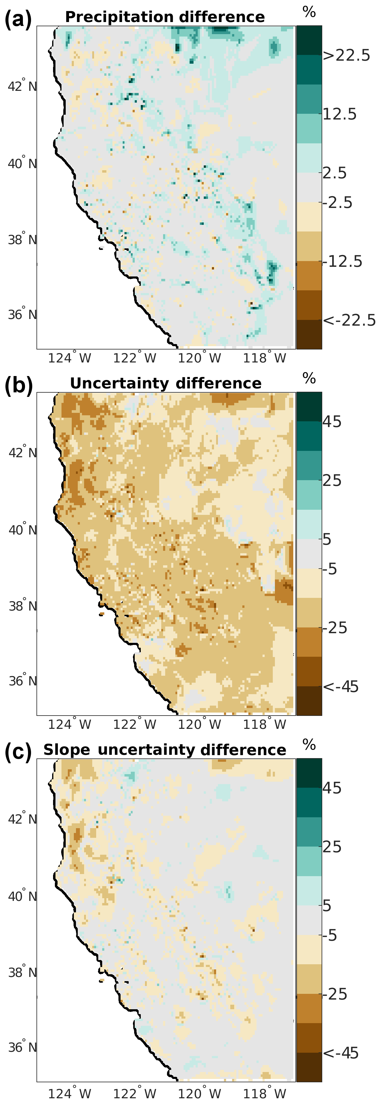
Figure 11Spatial distribution of differences for model parameter sensitivity experiment 3, modified maximum number of stations parameter (nMaxNear). (a) Precipitation differences (%), (b) total uncertainty differences (%), and (c) uncertainty changes due to the slope term in the regression.
Increasing the number of stations considered reduces the estimated uncertainty across nearly the entire domain (Fig. 11b–c). On average, there is a 2.1 mm (16 %) reduction in the domain mean uncertainty, with some grid cells having reductions >25 %. The large decreases are primarily in regions of complex terrain, and this is controlled by changes in the slope uncertainty estimate, (Fig. 11c). This change in total uncertainty is slightly larger than but opposite in sign to the parameter modification in experiment 2.
The Topographically InformEd Regression (TIER) software was developed for several reasons. First, the systems for spatial modeling of meteorological variables from in situ observations have matured to the point that they are complex systems with many methodological choices and model parameters. TIERv1.0 provides an initial implementation of a knowledge-based statistical modeling system based on D94, D02, D00, D07, and D08 with the capability to explore different methodological choices in a systematic fashion. The system is modular so that new knowledge-based ideas can be added to the regression model through including new weighting terms. Model parameters are also accessible to the user, allowing for parameter perturbation experiments. More broadly, this should be viewed as a first step towards development of flexible, open-source systems that include many of the commonly used spatial interpolation models so the community can more fully understand methodological choices in gridded meteorological product generation (e.g., Newman et al., 2019). Understanding how methods and model parameters interact and modify the final output is key to improving these systems.
The parameter experiments performed here provide three examples highlighting how minor changes to one model parameter impact the final spatial distribution. For example, modifying the coastal weight exponent results in a shift in placement of precipitation across the domain (Fig. 10) and systematic changes in the estimated uncertainty. Increasing the maximum number of stations considered for the interpolation results in systematic changes to the precipitation distribution and decreases the sharpness of the final field (Fig. 11). Also, the spatial gradients of precipitation and total uncertainty changes are of opposite sign for experiments 2 and 3. In general, parameter changes that act to increase localization will enhance gradients and uncertainty, while those that decrease localization or increase sample sizes will decrease gradients and uncertainty. This highlights that parameter interactions could play a role in the final result through positive or negative feedbacks. Finally, experiments 2 and 3 result in non-significant differences as compared to the base case, while the MAE between the modified parameter sets in experiments 2 and 3 results in statistically significant MAE differences. Given the ability to perform parameter sensitivity experiments in TIER, we reemphasize the need for novel evaluation methods including out-of-sample station networks (e.g., Daly, 2006; Daly et al., 2017; Newman et al., 2019) that are as independent from the input networks as possible and integrated validation methods using ancillary observations such as streamflow and other modeling tools such as hydrologic models (Beck et al., 2017; Henn et al., 2018; Laiti et al., 2018).
Finally, TIER does not implement the exact system developed by Daly and colleagues and will not produce the same climate fields even with the same input data. TIER is not duplicating source code and every feature described in D94, D00, D02, D07, and D08, as TIER was developed as a knowledge-based system following these papers, not replicating them and other unpublished details. Also, TIER version 1.0 does not contain station input data pre-processing routines. Instead, example input data are provided in the example cases' dataset (Sect. 5). Station pre-processing and quality control can encompass a vast number of methods (e.g., Serreze et al., 1999; Eischeid et al., 2000; Durre et al., 2008, 2010; Menne and Williams 2009). These methods may be included in future releases or as separate community station quality control tools.
The TIERv1.0 code is available at https://doi.org/10.5281/zenodo.3234938 (Newman, 2019a). The active development repository of TIER is located at https://github.com/NCAR/TIER (Newman, 2019b).
The input data for the example domain used here are available at https://ral.ucar.edu/solutions/products/the-topographically-informed-regression-tier-model (Newman, 2019c).
AJN and MPC developed the TIER model concept. AJN implemented the model and developed the test case, model validation, and model sensitivity experiments. AJN and MPC contributed to the manuscript.
The authors declare that they have no conflict of interest.
Color tables used here are provided by Wikipedia (precipitation), GMT (difference plots), and the GRID-Arendal project (http://www.grida.no/, last access: 17 November 2019) (temperature) via the NCAR NCL and cpt-city color table archives (https://www.ncl.ucar.edu/Document/Graphics/color_table_gallery.shtml, last access: 7 June 2019, http://soliton.vm.bytemark.co.uk/pub/cpt-city/, last access: 18 February 2017).
This research has been supported by the National Center for Atmospheric Research, which is a major facility sponsored by the National Science Foundation under cooperative agreement no. 1852977, and the US Army Corps of Engineers (USACE) Climate Preparedness and Resilience program.
This paper was edited by Richard Neale and reviewed by two anonymous referees.
Alter, J. C.: Normal precipitation in Utah, Mon. Weather Rev., 47, 633–636, 1919.
Banerjee, S., Gelfand, A. E., and Carlin, B. P.: Hierarchical Modeling and Analysis for Spatial Data, Boca Raton, FL, CRC Press, 2003.
Barnes, S. L: A technique for maximizing details in numerical weather map analysis, J. Appl. Meteorol., 3, 396–409, 1964.
Beck, H. E., Vergopolan, N., Pan, M., Levizzani, V., van Dijk, A. I. J. M., Weedon, G. P., Brocca, L., Pappenberger, F., Huffman, G. J., and Wood, E. F.: Global-scale evaluation of 22 precipitation datasets using gauge observations and hydrological modeling, Hydrol. Earth Syst. Sci., 21, 6201–6217, https://doi.org/10.5194/hess-21-6201-2017, 2017.
Chua, S. C. and Bras, R. L.: Optimal estimator of mean areal precipitation in regions of orographic influence, J. Hydrol., 57, 23–48, 1982.
Clark, M. P. and Slater, A. G.: Probabilistic quantitative precipitation estimation in complex terrain, J. Hydrometeorol., 7, 3–22, 2006.
Clark, M. P., Kavetski, D., and Fenicia, F.: Pursuing the method of multiple working hypotheses for hydrological modeling, Water Resour. Res., 47, W09301, https://doi.org/10.1029/2010WR009827, 2011.
Cornes, R. C., van der Schrier, G., van den Besselaar, E. J. M., and Jones, P. D.: An ensemble version of the E-OBS temperature and precipitation data sets, J. Geophys. Res.-Atmos., 123, 9391–9409, https://doi.org/10.1029/2017JD028200, 2018.
Cressie, N. and Wikle, C. K.: Statistics for Spatio-Temporal Data, New York, Wiley, 2011.
Daly, C.: Guidelines for assessing the suitability of spatial climate data sets, Int. J. Climatol., 26, 707–721, 2006
Daly, C., Neilson, R. P., and Phillips, D. L.: A Statistical-Topographic Model for Mapping Climatological Precipitation over Mountainous Terrain, J. Appl. Meteorol., 33, 140–158, 1994.
Daly, C., Taylor, G., Gibson, W., Parzybok, T., Johnson, G., and Pasteris, P.: High-quality spatial climate data sets for the United States and beyond, T. ASAE, 43, 1957–1962, 2000.
Daly, C., Gibson, W. P., Taylor, G. H., Johnson, G. L., and Pasteris, P.: A knowledge-based approach to the statistical mapping of climate, Clim. Res., 22, 99–113, https://doi.org/10.3354/cr022099, 2002.
Daly, C., Smith, J. W., Smith, J. I., and McKane, R. B: High-resolution spatial modeling of daily weather elements for a catchment in the Oregon Cascade Mountains, United States, J. Appl. Meteorol. Clim., 46, 1565–1586, 2007.
Daly, C., Halbleib, M., Smith, J. I., Gibson, W. P., Doggett, M. K., Taylor, G. H., Curtis, J., and Pasteris, P. A.: Physiographically-sensitive mapping of temperature and precipitation across the conterminous United States, Int. J. Climatol., 28, 2031–2064, https://doi.org/10.1002/joc.1688, 2008.
Daly, C., Slater, M. E., Roberti, J. A., Laseter, S. H., and Swift Jr., L. W.: High-resolution precipitation mapping in a mountainous watershed: ground truth for evaluating uncertainty in a national precipitation dataset, Int. J. Climatol., 37, 124–137, https://doi.org/10.1002/joc.4986, 2017.
Day, G. N: Extended streamflow forecasting using NWSRFS, J. Water Res. Pl., 111, 157–170, https://doi.org/10.1061/(ASCE)0733-9496(1985)111:2(157), 1985.
Durre, I., Menne, M. J., and Vose, R. S.: Strategies for eval- uating quality assurance procedures, J. Appl. Meteorol. Clim., 47, 1785–1791, https://doi.org/10.1175/2007JAMC1706.1, 2008.
Durre, I., Menne, M. J., Gleason, B. E., Houston, T. G., and Vose, R. S.: Comprehensive automated quality assurance of daily surface observations, J. Appl. Meteorol. Clim., 49, 1615–1633, https://doi.org/10.1175/2010JAMC2375.1, 2010.
Eischeid, J. K., Pasteris, P. A., Dias, H. F., Plantico, M. S., and Lott, N. J.: Creating a serially complete, national daily time series of temperature and precipitation for the western United States, J. Appl. Meteorol., 39, 1580–1591, 2000.
Franklin, J.: Predictive vegetation mapping: geographical modelling of biospatial patterns in relation to environmental gradients, Prog. Phys. Geog., 19, 474–499, 1995.
Henn, B., Clark, M. P., Kavetski, D., Newman, A. J., Hughes, M., McGurk, B., and Lundquist, J. D.: Spatiotemporal patterns of precipitation inferred from streamflow observations across the Sierra Nevada mountain range, J. Hydrol., 556, 993–1012, https://doi.org/10.1016/j.jhydrol.2016.08.009, 2018.
Houghton, J. G.: A model for orographic precipitation in the north-central Great Basin, Mon. Weather Rev., 107, 1462–1475, 1979.
Laiti, L., Mallucci, S., Piccolroaz, S., Bellin, A., Zardi, D., Fiori, A., Nikulin, G., and Majone, B.: Testing the hydrological coherence of high-resolution gridded precipitation and temperature data sets, Water Resour. Res., 54, 1999–2016, https://doi.org/10.1002/2017WR021633, 2018.
Liu, C., Ikeda, K., Rasmussen, R., Barlage, M., Newman, A. J., Prein, A. F., Chen, F., Chen, L., Clark, M., Dai, A., Dudhia, J., Eidhammer, T., Gochis, D., Gutmann, E., Kurkute, S., Li, Y., Thompson, G., and Yates, D.: Continental-scale convection-permitting modeling of the current and future climate of North America, Clim. Dynam., 49, 71–95, https://doi.org/10.1007/s00382-016-3327-9, 2017.
Livneh, B., Bohn, T. J., Pierce, D. W., Munoz-Arriola, F., Nijssen, B., Vose, R., Cayan, D. R., and Brekke, L.: A spatially comprehensive, hydrometeorological data set for Mexico, the U.S., and Southern Canada 1950–2013, Scientific Data, 5, 150042, https://doi.org/10.1038/sdata.2015.42, 2015.
Lundquist, J. D., Hughes, M., Henn, B., Gutmann, E. D., Livneh, B., Dozier, J., and Neiman, P.: High-elevation precipitation patterns: Using snow measurements to assess daily gridded datasets across the Sierra Nevada, California, J. Hydrometeorol., 16, 1773–1792, https://doi.org/10.1175/JHM-D-15-0019.1, 2015.
Menne, M. J. and Williams, C. N.: Homogenization of Temperature Series via Pairwise Comparisons, J. Climate, 22, 1700–1717, https://doi.org/10.1175/2008JCLI2263.1, 2009.
Newman, A. J.: The Topographically InformEd Regression (TIER) model version 1.0, https://doi.org/10.5281/zenodo.3234938, 2019a.
Newman, A. J.: Repository for the Topographically InformEd Regression (TIER) Model, available at: https://github.com/NCAR/TIER/, last access: 29 May 2019b.
Newman, A. J.: Test case for the Topographically InformEd Regression (TIER) Model, available at: https://ral.ucar.edu/solutions/products/the-topographically-informed-regression-tier-mode, last access: 29 May 2019c.
Newman, A. J., Clark, M. P., Craig, J., Nijssen, B., Wood, A., Gutmann, E., Mizukami, N., Brekke, L., and Arnold, J. R.: Gridded Ensemble Precipitation and Temperature Estimates for the Contiguous United States, J. Hydrometeorol., 16, 2481–2500, https://doi.org/10.1175/JHM-D-15-0026.1, 2015.
Newman, A. J., Clark, M. P., Longman, R. L., and Giambelluca, T. W.: Methodological Inter-Comparison of Gridded Precipitation and Temperature Products, J. Hydrometeorol., 20, 531–547, 2019.
Nychka, D., Bandyopadhyay, S., Hammerling, D., Lindgren, F., and Sain, S.: A multiresolution Gaussian process model for the analysis of large spatial datasets, J. Comput. Graph. Stat., 24, 579–599, 2015.
Pierce, D. W., Cayan, D. R., and Thrasher, B. L.: Statistical Downscaling Using Localized Constructed Analogs (LOCA), J. Hydrometeorol., 15, 2558–2585, https://doi.org/10.1175/JHM-D-14-0082.1, 2014.
Phillips, D. L., Dolph, J., and Marks, D.: A comparison of geostatistical procedures for spatial analysis of precipitation in mountainous terrain, Agr. Forest Meteorol., 58, 119–141, 1992.
Schermerhorn, V. P.: Relations between topography and annual precipitation in western Oregon and Washington, Water Resour. Res., 3, 707–711, 1967.
Serreze, M. C., Clark, M. P., Armstrong, R. L., McGinnis, D. A., and Pulwarty, R. L.: Characteristics of the western U.S. snowpack from snowpack telemetry (SNOTEL) data, Water Resour. Res., 35, 2145–2160, https://doi.org/10.1029/1999WR900090, 1999.
Shepard, D.: A two-dimensional interpolation function for irregularly-spaced data, Association for Computing Machinery, Proceedings of the 1968 23rd ACM National Conference, 517–524, 1968.
Shepard, D. S.: Computer mapping: The SYMAP interpolation algorithm, Spatial Statistics and Models, edited by: Gaile, G. L. and Willmott, C. J., D. Reidel, 133–145, 1984.
Smith, R. B. and Barstad, I.: A Linear Theory of Orographic Precipitation, J. Atmos. Sci., 61, 1377–1391, https://doi.org/10.1175/1520-0469(2004)061<1377:ALTOOP>2.0.CO;2, 2004.
Spreen, W. C: A determination on the effect of topography upon precipitation, T. Am. Geophys. Un., 28, 285–290, 1947.
Thiessen, A. H.: Precipitation averages for large areas, Mon. Weather Rev., 39, 1082–1084, 1911.
Thornton, P. E., Running, S. W., and White, M. A.: Generating surfaces of daily meteorological variables over large regions of complex terrain, J. Hydrol., 190, 214–251, https://doi.org/10.1016/S0022-1694(96)03128-9, 1997.
Thornton, P. E., Thornton, M. M., Mayer, B.W., Wei, Y., Devarakonda, R., Vose, R. S., and Cook, R. B.: Daymet: Daily Surface Weather Data on a 1-km Grid for North America, Version 3, ORNL DAAC, Oak Ridge, Tennessee, USA, https://doi.org/10.3334/ORNLDAAC/1328, 2018.
United States Bureau of Reclamation (USBR): Colorado River Basin Water Supply and Demand Study, U.S. Department of the Interior, Bureau of Reclamation, 1697 pp., available at: https://www.usbr.gov/lc/region/programs/crbstudy.html (last access: 1 March 2017), 2012.
Willmott, C. J. and Matsuura, K.: Smart Interpolation of Annually Averaged Air Temperature in the United States, J. Appl. Meteorol., 34, 2577–2586, https://doi.org/10.1175/1520-0450(1995)034<2577:SIOAAA>2.0.CO;2, 1995.
Willmott, C. J. and Robeson, S. M.: Climatologically aided interpolation (CAI) of terrestrial air temperature, Int. J. Climatol., 15, 221–229, 1995.
Xia, Y., Mitchell, K., Ek, M., Sheffield, J., Cosgrove, B., Wood, E., Luo, L., Alonge, C., Wei, H., Meng, J., and Livneh, B.: Continental-scale water and energy flux analysis and validation for the North American Land Data Assimilation System project phase 2 (NLDAS-2): 1. Intercomparison and application of model products, J. Geophys. Res., 117, D03109, https://doi.org/10.1029/2011JD016048, 2012.