the Creative Commons Attribution 4.0 License.
the Creative Commons Attribution 4.0 License.
 | 09 Apr 2020
SICOPOLIS-AD v1: an open-source adjoint modeling framework for ice sheet simulation enabled by the algorithmic differentiation tool OpenAD
Liz C. Logan
Sri Hari Krishna Narayanan
Ralf Greve
We present a new capability of the ice sheet model SICOPOLIS that enables flexible adjoint code generation via source transformation using the open-source algorithmic differentiation (AD) tool OpenAD. The adjoint code enables efficient calculation of the sensitivities of a scalar-valued objective function or quantity of interest (QoI) to a range of important, often spatially varying and uncertain model input variables, including initial and boundary conditions, as well as model parameters. Compared to earlier work on the adjoint code generation of SICOPOLIS, our work makes several important advances: (i) it is embedded within the up-to-date trunk of the SICOPOLIS repository – accounting for 1.5 decades of code development and improvements – and is readily available to the wider community; (ii) the AD tool used, OpenAD, is an open-source tool; (iii) the adjoint code developed is applicable to both Greenland and Antarctica, including grounded ice as well as floating ice shelves, with an extended choice of thermodynamical representations. A number of code refactorization steps were required. They are discussed in detail in an Appendix as they hold lessons for the application of AD to legacy codes at large. As an example application, we examine the sensitivity of the total Antarctic Ice Sheet volume to changes in initial ice thickness, austral summer precipitation, and basal and surface temperatures across the ice sheet. Simulations of Antarctica with floating ice shelves show that over 100 years of simulation the sensitivity of total ice sheet volume to the initial ice thickness and precipitation is almost uniformly positive, while the sensitivities to surface and basal temperature are almost uniformly negative. Sensitivity to austral summer precipitation is largest on floating ice shelves from Queen Maud to Queen Mary Land. The largest sensitivity to initial ice thickness is at outlet glaciers around Antarctica. Comparison between total ice sheet volume sensitivities to surface and basal temperature shows that surface temperature sensitivities are higher broadly across the floating ice shelves, while basal temperature sensitivities are highest at the grounding lines of floating ice shelves and outlet glaciers. A uniformly perturbed region of East Antarctica reveals that, among the four control variables tested here, total ice sheet volume is the most sensitive to variations in austral summer precipitation as formulated in SICOPOLIS. Comparison between adjoint- and finite-difference-derived sensitivities shows good agreement, lending confidence that the AD tool is producing correct adjoint code. The new modeling infrastructure is freely available at http://www.sicopolis.net (last access: 2 April 2020) under the development trunk.


An important ingredient to characterizing and quantifying our uncertainty in expected climate change outcomes is our understanding of ice sheet dynamics. A key approach for increasing such understanding is the development of more sophisticated ice sheet models. Scientists have made significant strides in improving model sophistication, with the latest class of ice sheet models resolving all three dimensions of the ice sheet's internal stress balance (as opposed to previous classes of models, which employed various approximations to the stress field to save computational cost). However, while advances in computational glaciology have enabled us to simulate ice sheet behavior more accurately, remaining uncertainties in the range of independent input variables required for ice sheet simulations, in particular initial conditions, surface forcings, basal boundary conditions, and internal parameters, comprise crucial weaknesses in ice sheet – and ultimately climate system – prediction or projection (Goelzer et al., 2018; Seroussi et al., 2019). As such, ice sheet modeling is facing similar issues of robust model initialization for prediction as those faced by the climate modeling community at large (e.g., Meehl et al., 2014; Balmaseda, 2017).
Ice flow critically depends on quantities that we either cannot easily measure (such as the friction or thermal forcing between ice and the bedrock below it), that parameterize subgrid-scale processes or empirical constitutive laws (such as the routing of meltwater or fracture propagation), or that we may never be able to measure in the present day (such as the rate of snowfall in the past). These unknown or uncertain variables can be construed as sets of parameters that we must infer or calibrate if we are to make projections with ice sheet models, and these parameters must both satisfy, by some measure, the assumed model physics and the sparsely made observations across such large bodies. In the language of optimal estimation and control theory, these parameters are referred to as control variables (Gelb, 1974).
If we are to integrate ice sheet model projections into societally relevant discussions on sea level rise, we may wish to know the sensitivity of ice-sheet-integrated or derived quantities of interest to a range of uncertain model inputs. For example, we wish to know how the total ice volume (above flotation) of an ice sheet is influenced by climatically relevant quantities (such as surface atmospheric forcings) or environmental variables (such as the melting at the base of an outlet glacier or floating ice shelf that drains an ice sheet). A computationally costly method for deriving such sensitivities might use individually made perturbations to the bottom melting rate at each location of the ice sheet’s base, in particular at its margins that are in contact with ocean water. This means that the ice sheet dynamics must be integrated throughout time for each simulation experiment in which a point-wise perturbation has been applied in order to assemble a sensitivity map across the entire domain to this control variable (basal melting). While the target of this approach remains of paramount importance – relating the output of an ice sheet model to poorly known inputs – the means are computationally expensive: understanding, for instance, the Antarctic Ice Sheet’s sensitivity to changes in melting or basal friction means simulating the entire ice sheet throughout time for every perturbation made at each point in the domain. In this case the computational cost of such a method scales with the dimension of the domain grid, and as such it is prohibitive.
Fortunately, adjoint models provide us with a means to this end whereby the computational cost of deriving sensitivity maps does not depend on the dimension of the control variable space. The adjoint model is in effect the transpose of the linearized operator of the ice sheet model. Compared to the parent model, which propagates model inputs via the prognostic model state to model outputs, the adjoint propagates the dual of the ice sheet model state in reverse order, from the sensitivity of model outputs to sensitivities in the model inputs (which, for time-dependent models, amounts to a backward-in-time propagation of sensitivities). It thereby simultaneously calculates the sensitivity of a chosen quantity of interest (e.g., the volume of an ice sheet) with respect to the prescribed set of control variables (e.g., the basal melting beneath the ice, surface accumulation, or initial conditions). Thus, unlike the tangent linear model, which computes the impact of one input perturbation on all model outputs at the cost of one execution (directional derivative), the adjoint model computes the sensitivity of one output quantity of interest (QoI) with respect to all model inputs (gradient). This is useful not only for understanding the sensitivity of some scientifically or societally interesting quantity to model inputs, but further (and perhaps more interesting) enables the recovery of other forcing or initial conditions (e.g., initial ice sheet geometry or rate of snow accumulation throughout time and space) through formal inversion.
1.1 Algorithmic differentiation (AD) and its uses
Generally, adjoint models arise in at least two classes of geophysical investigations.
1.1.1 PDE-constrained, gradient-based optimization
Adjoint-enabled optimization problems that are constrained by partial differential equations (PDEs), which are solved by using adjoint methods, may be posed in the following manner, beginning by formulating a scalar-valued cost function based on a least-squares model–data misfit subject to prior information on the uncertainty of the control variables:
where x0, xb, and x(ti) are the initial, background, and time-varying model state at time ti, respectively; yi is the set of observations at time ti and Ei(x(ti)) is a projection of the model state at time ti to space of observations yi (or the data–model misfit). Cpr is a prior error covariance matrix (usually diagonal as its structure is not fully known), and Cerr is an observational error covariance matrix. This form is typical for a problem in which uncertain initial conditions are subject to variation to reduce the model–data misfit, and with prior information available (xb and Cpr). The formulation may be readily extended to include variation of boundary conditions or model parameters, and the collective set of all such input variables that are being subject to variation are called control variables (see Wunsch and Heimbach, 2007, for a more comprehensive treatment).
PDE-constrained optimization seeks to find the gradient of 𝒥 with respect to the control variables (here x0), subject to the requirement that the (in general nonlinear) model ℒ is fulfilled, rendered by a set of partial differential equations that step the state x from time ti to ti+1, i.e.,
This problem is efficiently solved by means of the Lagrange multiplier method (Wunsch and Heimbach, 2007). Lagrange multipliers have a direct interpretation as dual-state adjoint sensitivities or gradients of the cost function (Eq. 1) with respect to the control variables, . They are used to seek a state of the system, x∗, that is tolerably close to the minimum of 𝒥. As such, gradient information is essential in recovering the optimal x∗, which minimizes model–data misfit as presented by Eq. (1). This procedure is done in an iterative fashion, with an initial guess of the state x0 that is successively updated to achieve optimal control variables that produce an optimal prognostic model state throughout the model's simulation.
A model that can optimally reproduce the behavior of, e.g., an ice sheet throughout time with respect to observations possesses the advantage that model-derived predictions might be made with greater confidence, having been initialized by dynamics that are informed by spatiotemporal observations. In other words, the commonly termed “spin-up” of an ice sheet may produce more faithful projections when forced by optimally recovered initial and boundary conditions, and an optimal state estimate, which may be recovered by a time-dependent adjoint model. A model initialized and projected under such circumstances might better reproduce what can be inferred about its past state by observations, subject to the additional constraint of the assumed and (perhaps more subtle, but equally important) conserved model physics throughout time. Thus, the constrained optimization problem of recovering boundary and initial conditions, and the model's optimal internal state dynamics throughout space and time, might be approached first through the task of obtaining reliable adjoint sensitivities.
1.1.2 Sensitivity analysis
Beyond applications in optimization, the adjoint may also be widely applied to the comprehensive analysis of linear sensitivities (the subject of the work presented here) of QoIs to uncertainly known inputs (in particular, forcings or parameters) in nonlinear models. Errico and Vukicevic (1992) and Marotzke et al. (1999) provide example applications in the context of atmosphere and ocean modeling, respectively. For a general scalar-valued function 𝒥, now termed the quantity of interest (QoI), the tangent linear model (TLM) L of a given (in general nonlinear) model ℒ (Eq. 2) acts as a directional derivative, as it propagates small perturbations in the control variable, δx, to corresponding perturbations in the QoI, δ𝒥. In turn, the adjoint model (ADM), formally the transpose LT of the tangent linear model, propagates the sensitivities of the QoI to each component of the control space, i.e., the partial derivatives of the augmented space of all control variables in reverse order of the execution of the forward model ℒ (which, for time-dependent models, amounts to the integration backward in time of the adjoint model equations). Thus, whereas the TLM produces directional derivatives of 𝒥, the adjoint produces the gradient of 𝒥. A detailed treatment in the context of ice sheet modeling is provided by Heimbach and Bugnion (2009) and Goldberg and Heimbach (2013). For the present purpose we summarize the way in which these sensitivities are formally obtained by way of algorithmic differentiation in the following.
1.2 Formal reverse mode of AD
The concept of the adjoint of a numerical model may be best understood in terms of the forward, original code construction and execution. If one wishes to know the sensitivity of some QoI (e.g., the volume of the Antarctic Ice Sheet) with respect to some model inputs or control variable (e.g., the average surface air temperature in July), one method of pursuing knowledge about such a sensitivity might be perturbing the control variable, in sequence, at each single point within the discretized domain and propagating the perturbation forward in time. The perturbation to the control variable results in a change in the QoI, and one can proceed to calculate the sensitivity of the QoI with respect to the control variable everywhere in the domain. Herein these are termed the finite differences of the QoI 𝒥 with respect to the (in general vector-valued) control variable x in the direction Δx, where 𝒥 is calculated as in Eq. (1). An adjoint model code may be demonstrated as acceptable or reliable if the finite-difference-derived sensitivities approximate the adjoint-derived sensitivities (within some tolerance); for example, for a centered finite difference we obtain
where ε is the magnitude of the perturbation to the control and is the unit vector pointing in the direction of δx. In this work ε varies depending on the examined control. Other finite-difference schemes may of course be employed, but for the purposes of this work we have selected the central difference for simplicity.
Adjoint models have been common in oceanic and atmospheric contexts (Talagrand and Courtier, 1987; Thacker and Long, 1988; Errico and Vukicevic, 1992) for decades. The method's popularity has been increasing steadily. MacAyeal et al. (1991) provide us with the earliest use of adjoint-model-derived sensitivities of a simplified ice stream model. Observed velocities were used to invert for optimal basal friction parameters. While that study employed a simplified version of the Stokes equations and lacked time dependence, other researchers have since undertaken the task of using adjoint sensitivities in a variety of ice-related applications with more complexity. Inversions of basal (Gillet-Chaulet et al., 2012; Goldberg and Sergienko, 2011; Joughin et al., 2009; Morlighem et al., 2010, 2013; Vieli and Payne, 2003) and rheological (Larour et al., 2005; Khazendar et al., 2007) parameters were produced based on regional implementations of steady-state models of the Antarctic Ice Sheet, with varying degrees of approximations to the internal stress balance. Brinkerhoff and Johnson (2013) and Perego et al. (2014) used the method with an emphasis on producing optimal initial conditions for prediction. Waddington et al. (2007) provide one of the few examples to date for inferring surface boundary conditions (accumulation rates) from internal radar layer observations. The extended problem of inversion in the context of transient ice sheet models was considered by Goldberg and Heimbach (2013), Goldberg et al. (2015, 2016), and Larour et al. (2014). Use of higher-order derivatives (in particular, Hessian) to extend the inverse problem to the problem of quantifying uncertainties in the inferred parameters was treated by Petra et al. (2012) and Isaac et al. (2015). Mosbeux et al. (2016) provided an intercomparison of two assimilation methods for inferring basal parameters by comparing a sequential and an adjoint approach.
Compared to the literature cited above, and specifically in contrast to the work by Heimbach and Bugnion (2009) and Goldberg and Heimbach (2013), our work presents several technical (model development) and scientific (application of the capability developed) novel aspects:
-
we develop the capability to generate the adjoint of a thermomechanically coupled ice sheet model by means of source-to-source transformation algorithmic differentiation (AD) using an open-source AD tool;
-
the code for source-to-source transformation is the an up-to-date version of the SICOPOLIS model, which should enable easy maintenance of the AD capability and wider use by the interested research community;
-
compared to Heimbach and Bugnion (2009) the current SICOPOLIS model (5-dev) has several choices of thermodynamic representations and the ability to augment the shallow-ice approximation for grounded ice with a shallow-shelf approximation for ice floating in the ocean. This study will derive continent-wide sensitivities of changes in Antarctic ice volume to changes in sub-ice-shelf melt rates.
An inherent problem in the numerical simulation of ice dynamics is the nonlinearity of the forward model. This arises due to the nonlinear dependence of viscosity on a stress or strain rate formulation in ice. Because of this complication, hand-coded adjoints can be as labor-intensive (and error-prone) to develop as their nonlinear parent model. As an alternative to hand-coding the adjoint model, algorithmic differentiation (AD) provides a method for obtaining adjoint codes via rigorous exploitation of the chain (and product) rule (Griewank and Walther, 2008; Forth et al., 2012; Naumann, 2012) (http://www.autodiff.org, last access: 2 April 2020). AD has been used in an array of applications in the geosciences and computational fluid dynamics and has one substantive advantage over handwritten adjoint codes: it is flexible. Changes in the prescribed QoI, the control variables, or the underlying assumed and discretized model physics may lead to adjoint models of different structure. As models become more complicated due to time dependence and the inclusion of improved representation of ice physics, accurate, hand-coded adjoint solutions may be even more difficult to derive. In such contexts, AD methods provide a powerful alternative means for producing adjoint solutions to time-dependent problems that are up to date with respect to their parent forward model code.
Adjoint models developed by AD exploit the chain and product rules for the computation of the derivatives of a function (𝒥) with respect to a set of input variables (u). For simplicity, here we only consider the case in which the control variables consist of the initial state of the model, (for a complete treatment, see Wunsch and Heimbach, 2007). To demonstrate how a scalar QoI, 𝒥, is related to a control vector u, consider the following time-dependent statement of the problem, where represents marching the model forward through discretized time steps:
where x(tf) is the model's state at the end of the simulation, ℒ represents the overall mapping of the control vector to the final state of the model, and ℒ is the nonlinear system of equations (or forward model) applied successively to the initial state of the model. The subscripting of ℒ refers to the time marching of the model, where tf=Δt Nt, and ℒn maps the model state at time n to n+1. As our interest here is to show how gradients are generated by this method, consider then how linear perturbations to the control space result in changes to the cost function, 𝒥, through a Taylor series expansion:
Assuming 𝒪(δ𝒥2) is negligible, and considering another simplifying case in which 𝒥 only depends explicitly on the final state x(tf), δ𝒥 is shown (in the forward sense) to be
where is the inner product and is the tangent linear model of ℳ, a linearization of ℒ at time tn about x0. It follows from Eq. (6) that the adjoint model LT(where LT is the transpose of L) equivalently defines δ𝒥:
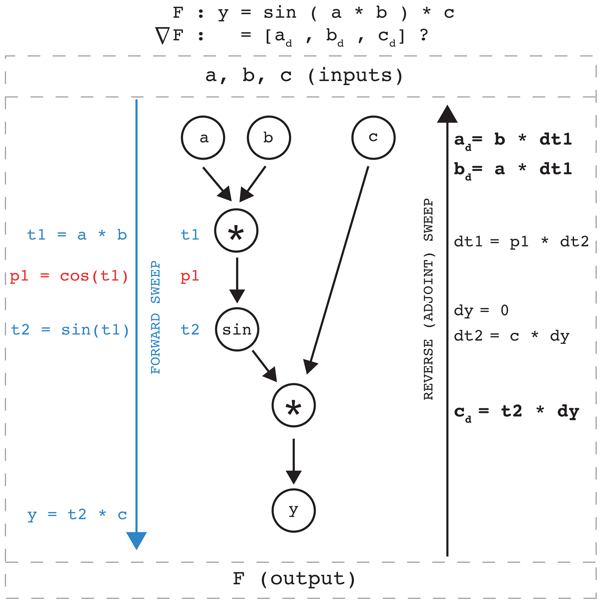
Figure 1Schematic of AD applied to a simple function, (see top). Intermediate results of the function evaluation are
stored in the intermediate variables t1 and t2.
We wish to determine the gradient of ℱ with respect to all inputs a,b, and c, symbolically expressed as
.
In SICOPOLIS-AD, the entire forward code is composed of many lines of simple functions, like ℱ, in sequence (blue downward-pointing array on the left). OpenAD provides ∇ℱ by relating the partials of t1 and t2 to intrinsically differentiable functions, like sin(), here the red text, p1 (black upward-pointing array on the right).
The partial derivatives of ℱ are computed via the writing to memory of intermediate partial quantities, like dy (the adjoint or dual of y) , dt1, and dt2. Thus, the sought sensitivity of a QoI, ℱ, is related to input parameters a, b, and c in this algorithmic (albeit much simplified) manner.
Equation (7) demonstrates that the sought gradient, , is computed by projecting the cost function to the model's final state, , and mapping it backward in time, ultimately to the dependence of the model on its (user-selected) input or control variables. Figure 1 presents a small example of the computational flow of the full nonlinear forward sweep (blue arrow and variables) and the adjoint (reverse) mode of OpenAD (black arrow) applied to a single model, , where the gradient of is sought (see Heimbach and Bugnion, 2009, for a related schematic of the relationship between forward and adjoint code via source-to-source transformation AD).
As soon as a numerical model is implemented as a code, it is in fact translated as a sequence or composition of elementary operations like those shown in Fig. 1, with a single line representing one single algorithmic step. Via AD methods, then, the tangent linear and adjoint of a numerical model are provided by exhaustive application of the chain and product rules, line by line, to the model. The forward (Sect. 2.1) or reverse (adjoint) mode of the model may be thought of as the composition in forward or reverse order of the Jacobian matrices and their transpose of the full forward code's line-by-line algorithmic elements: that is, L in Eq. (6) and LT in Eq. (7).
2.1 Forward model SICOPOLIS
We begin with the ice sheet model SICOPOLIS (SImulation COde for POLythermal Ice Sheets) and sketch the development of its adjoint model from version 5-dev (Greve, 2019; Rückamp et al., 2019) (http://www.sicopolis.net, last access: 2 April 2020). SICOPOLIS is open source and written in Fortran; it has a relatively long and stable history (Greve, 1997). SICOPOLIS has remained a relevant and powerful tool for the cryosphere community and continues to participate in model intercomparison exercises (e.g., Goelzer et al., 2018; Seroussi et al., 2019). The model couples ice sheet dynamics and thermodynamics (solving for the ice thickness, extent, velocity, temperature, water content, and age) over three-dimensional domains including, among others, Greenland, Antarctica, paleo-ice sheets on Earth, and the polar caps of Mars. It employs simplified versions of the three-dimensional Stokes equation (internal stress balance). These include the shallow-ice approximation for ice resting on land (Hutter, 1983; Morland, 1984), the shallow-shelf approximation for ice floating in the ocean (Morland, 1987; MacAyeal, 1989; Weis et al., 1999), and the shelfy-stream approximation for fast-flowing ice streams with limited coupling to the bed (Bernales et al., 2017). For a detailed treatment of the numerical methods employed in the model, readers are referred to Greve and Calov (2002), Greve and Blatter (2009, 2016), and Bernales et al. (2017).
SICOPOLIS employs four different thermodynamics representations: (1) a two-layer polythermal scheme, which allows for the computation and effects of liquid water within a warmer temperate layer; (2) a purely cold-ice scheme in which no liquid water is present; and (3, 4) two flavors of the one-layer enthalpy scheme that combine the physical adequateness of (1) with the greater numerical simplicity of (2) (Aschwanden et al., 2012; Greve and Blatter, 2016). In all cases, horizontal diffusion of the thermodynamic fields (temperature, water content, or enthalpy) is neglected. The solvers employed use an implicit discretization scheme for the vertical derivatives and an explicit scheme for the horizontal derivatives.
SICOPOLIS simulates ice as a nonlinear viscous fluid by employing Glen's flow law (Glen, 1955) amended as in Greve and Blatter (2009):
where η is the ice viscosity, T′ is the temperature difference relative to the pressure-melting point, σe is the effective shear stress, and σ0 is a small constant used to prevent singularities when σe is very small. n is the flow law exponent (taken as 3), and A is a temperature- and pressure-dependent rate factor (Cuffey and Paterson, 2010) that is modified in temperate regions containing liquid water following Lliboutry and Duval (1985).
Basal sliding under grounded ice links the sliding velocity, vb, to the basal shear traction, τb, and the basal normal stress, Nb (counted positive for compression), in the form of a Weertman–Budd-type sliding law (e.g., Weertman, 1964; Budd et al., 1984):
where Cb is the sliding coefficient, and p and q are the sliding law exponents.
2.2 Adjoint model of SICOPOLIS generated with OpenAD
As described in Sect. 1.1, the construction of an adjoint model of a nonlinear, time-dependent forward model often presents a formidable task when solved analytically or hand-coded (e.g., Goldberg and Sergienko, 2011; Gillet-Chaulet et al., 2012; Morlighem et al., 2013; Isaac et al., 2015). In previous works, the variational forward and adjoint equations are derived first and then discretized. As an alternative, AD produces adjoint code through the differentiation of source code using source transformation or operator overloading tools. As the standard of numerical models (in various contexts) has risen to more complicated physical representations, the use of AD has become increasingly popular (e.g., Heimbach and Bugnion, 2009; Goldberg et al., 2016; Hascoët and Morlighem, 2018, using source transformation – Brinkerhoff and Johnson, 2013; Larour et al., 2014; Hoffman et al., 2018, using operator-overloading and code-templating).
The adjoint of the ice sheet model SICOPOLIS is largely generated automatically by the application of the freely available source transformation tool OpenAD (Utke et al., 2008) developed at Argonne National Laboratory, the University of Chicago, and Rice University (http://www.mcs.anl.gov/OpenAD, last access: 2 April 2020). It is a flexible and modular tool that parses a given model written in Fortran to generate a Fortran version of the model's adjoint code. As opposed to adjoint models that are analytically derived and discretized, the adjoint model of SICOPOLIS furnished by AD yields not one unique adjoint code but many possible configurations of the adjoint model, whose constituent parts are selected at compile time by options in the header files. Thus, there no single, core adjoint code; there is instead a flexible adjoint code that evolves in tandem with the forward model of SICOPOLIS and can accommodate updated empirical relationships and boundary conditions.
The adjoint model of SICOPOLIS produced by OpenAD results in approximately 50 000 executable lines, represented in a much simplified schematic in Fig. 1 by the composition of the blue, red, and black algorithmic steps. Like many complex, time-evolving geophysical models, SICOPOLIS comes with a range of choices of model configuration, in particular numerical schemes, which the user may choose from. As a matter of convenience, the preferred implementation is to make all of these choices (or options) available at runtime to minimize the need for recompiling the model. The same convenience is available, in principle, to the AD-generated adjoint model. The control flow analysis of the AD tool identifies all possible flows of forward model execution and produces corresponding adjoint flow paths. However, close to 2 decades of experience with the application of AD to complex, time-evolving geophysical models, all of which have a range of numerical schemes that users may choose from (Heimbach et al., 2002, 2005; Forget et al., 2015), has shown that for the specific application of adjoint modeling, it is preferable to remove code that will not be executed in a given application from adjoint code generation (and subsequent compilation). The two main reasons for proceeding in this manner are the following.
- i.
The exclusion of forward model code that the user knows will not be executed may significantly simplify the AD tool's dependency and flow control analysis, avoid spurious dependencies that the AD tool may detect, and lead to more streamlined source code for the adjoint.
- ii.
Because of the reverse mode and requirement to store required variables in time-reversed order (e.g., those used for evaluating state-dependent conditions and nonlinear expressions), adjoint models will have a substantially larger memory footprint than their parent forward model (Heimbach et al., 2005). Memory requirements may be significantly increased if the adjoint model is required to keep track of a large range of conditional branches for execution.
For these practical considerations, removing nonused forward model code at the time of adjoint code generation and subsequent compilation has proven to be highly preferable (although not strictly required). It is implemented here via C preprocessor (CPP) options that are enabled or disabled prior to generating the adjoint code (and prior to compilation time). We note that the implementation keeps runtime parameters and flags in place such that the forward model default to keep all code available at runtime is not compromised. By pairing SICOPOLIS with the source transformation tool OpenAD, the adjoint model of SICOPOLIS may be generated automatically for a large variety of forward model configurations (including detailed choices of model domain, numerics, control variables, and QoI).
A number of algorithmic aspects of the code needed one-time editing or refactoring for OpenAD to be able to successfully parse the source code and provide correct adjoint code. For example, non-smooth functions – such as piecewise linear functions represented by if statements or absolute values – are inherently non-differentiable and sometimes required special treatment before the adjoint could be obtained by AD.
Because of its importance in the development of a forward model that works properly within the framework of the AD tool, we have devoted a detailed description in Appendix B of the aspects of SICOPOLIS that required code refactoring. Further technical details on how to set up, compile, and run reference configurations are documented in a quick-start manual (Logan et al., 2019).
Because SICOPOLIS is capable of simulating many different aspects of ice flow at the continental scale, we have designed a set of configurations each focusing on particular aspects of the model so that the resulting adjoint values and patterns may be more readily interpreted. Where we could have applied more complicated relationships, for example in the initialization in temperature, geothermal flux, or calving laws, we have opted instead for simplicity, as the exhaustive examination of such choices in simulation is left to future studies. The adjoint values are calculated for specific configurations of the original forward code of SICOPOLIS.
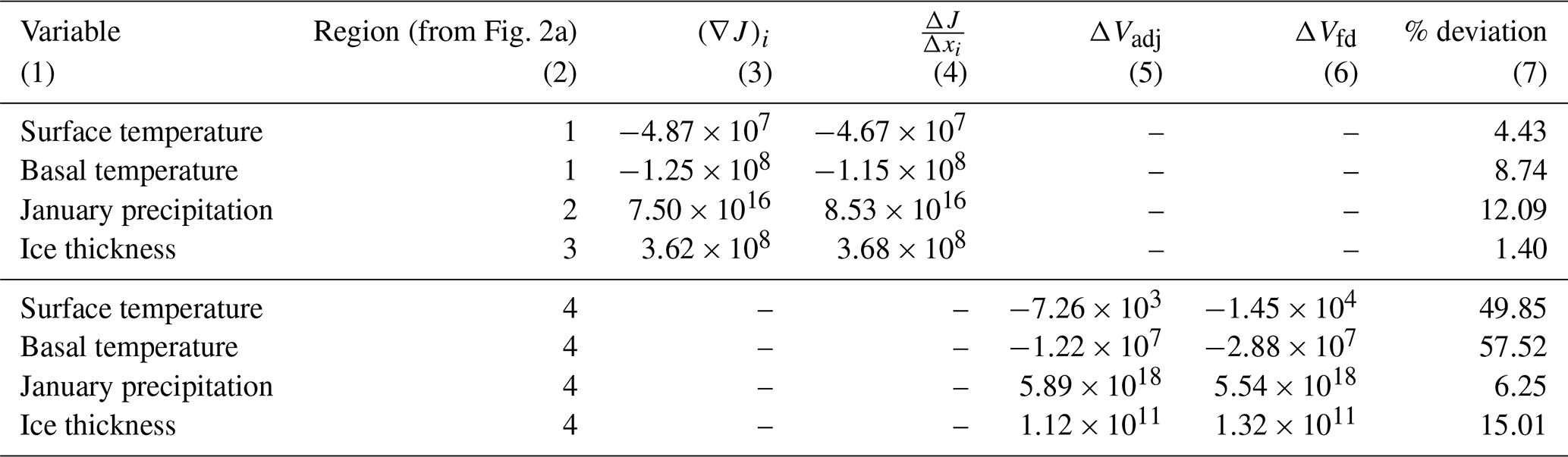
Table 1A sample of comparisons between adjoint-derived and finite-difference-based sensitivities. All regions in column (2) refer to either selected point-wise perturbations δxi=ϵ ei (with unit vector ei of the ith component) or perturbations applied over an extended box delineated in Fig. 1a. Columns (3) and (5) are adjoint-derived quantities, while columns (4) and (6) are derived via finite-difference perturbations either at a single point in the domain or integrated over a patch, as shown in Fig. 2a. Validation of the adjoint model is sought by comparing finite differences (4) and adjoint values (3) in a percent deviation metric (7). Column (7) is calculated as . Point-wise ice thickness as well as surface and basal temperatures compare well, with a percent deviation of less than 10 %. Summer precipitation has a higher disagreement, at 12 %. Patch-wide comparisons have a considerably higher percent deviation. We also performed a test for the Greenland Ice Sheet, shown in more detail in Appendix A.
3.1 Antarctic model configuration
We simulate Antarctica for 100 years of model time with a 20 km horizontal resolution and 81 terrain-following vertical layers. The dynamic and thermodynamic time steps (which can be chosen to differ) were both set to 0.2 years, as this was found to be the most stable value for the forward model simulation. Land ice, floating ice, and ice streams are approximated by the shallow-ice approximation (SIA), shallow-shelf approximation (SSA), and shelfy-stream approximation (SStA) formulations, respectively, described in Bernales et al. (2017). Ice thickness evolves freely and without adjustment. Solutions to the SSA portion of SICOPOLIS are aided by invoking the external Library of Iterative Solvers (LIS; https://www.ssisc.org/lis/, last access: 2 April 2020). Thermodynamics are formulated by the conventional enthalpy scheme (Sect. 2.1). We use Glen's flow law (Eq. 8) with a stress exponent n=3, a residual stress σ0=104 Pa, uniform flow enhancement factors E=5 for grounded ice and E=1 for floating ice, and a rate factor A(T′) as in Cuffey and Paterson (2010). Horizontal and vertical advection in the temperature and age equations are discretized via a first-order upstream stencil of interpolated velocities and advection terms on the main grid, and topography gradients are evaluated with a fourth-order discretization. The ice temperature is initialized as a uniform value of −10 ∘C, as the goal of this exercise is a proof of concept and not an exhaustive examination of all aspects of the Antarctic Ice Sheet. For the same reason, a uniform geothermal flux of 55 m W m−2 is applied. Parameterization of the mean annual and mean January surface temperatures is according to Fortuin and Oerlemans (1990), and the applied surface temperature is held constant throughout the simulation. Accumulation is applied at present-day levels throughout the simulation (Le Brocq et al., 2010; Arthern et al., 2006). The fraction of solid precipitation is a linear function of the monthly mean surface temperature according to Marsiat (1994). Surface ablation is parameterized by the positive degree day method, and rainfall is assumed to run off instantly. Floating ice is removed at calving fronts for thicknesses less than 30 m. The parameters for the basal sliding law (Eq. 9) are chosen as Cb=11.2 m yr−1 Pa−1, p=3, and q=2. Basal melting under floating ice is set to 30 m water equivalent per year around the grounding zone (adjacent grounded and floating grid points) and zero elsewhere, for simplicity. Sea level is constant, and there is no special treatment of subglacial hydrology. The initial geometry is taken from the present day (Fretwell et al., 2013). No isostatic bedrock adjustment is simulated in our configuration. No special pretreatment or “spin-up” of the model is applied prior to the 100-year simulation; rather, the above conditions are set and the model evolves for 100 years.
We note that the operation underlying calving (see above) amounts to a conditional statement. From an AD perspective, the following steps occur: (i) derivative codes are generated for each condition; (ii) code to store and restore the required variable is added to properly evaluate the conditional derivative. For legacy code the operation may not be differentiable at the exact condition (see Appendix B for practical details). This should be taken into account when performing gradient-based optimization.
3.2 Results
The motivation for developing an adjoint of a numerical model stretches far beyond providing comprehensive sensitivity experiments; often, an adjoint model is developed so that the sensitivities may be used in a gradient-based PDE-constrained optimization problem to invert for uncertain initial conditions, boundary conditions, or model parameters, thereby producing a data-constrained estimate for the evolution of the state of the system. Here, however, we are interesting in understanding model sensitivities. We present the sensitivity of the volume of the Antarctic Ice Sheet with respect to several control variables as a proof of concept, rather than extending the work in the direction of optimization, which will be the subject of future studies. The purpose is to gain physical insight into the model's linear response characteristics and to ascertain correctness and interpretability of the adjoint. The adjoint-derived sensitivities are compared to finite-difference perturbations, either at single points or over a patch of the domain that has been uniformly perturbed, to demonstrate that the adjoint model is sufficiently consistent with sensitivities derived via finite differences. Those comparisons are shown in Table 1. Lastly, compared to Heimbach and Bugnion (2009), we present this work for the novel application of examining Antarctic-wide adjoint-generated sensitivity maps. To the authors' knowledge, such a presentation has not been formally examined heretofore.
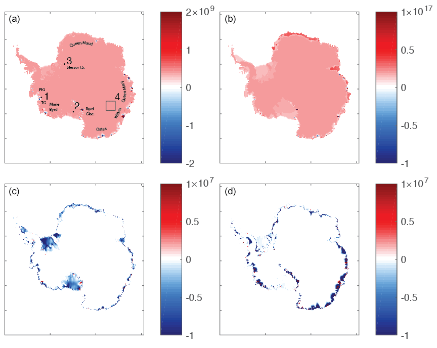
Figure 2Adjoint sensitivities, , for the Antarctic Ice Sheet, where Xi is the control variable shown. Control variables are the (a) initial ice thickness (m2), (b) mean January precipitation (m2 yr), (c) surface temperature (m3 ∘C−1), and (d) basal temperature (m3 ∘C−1). Locations in (a) numbered 1–4 are compared to finite-difference values in Table 1.
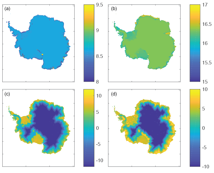
Figure 3Logarithms of the absolute value of adjoint sensitivities, , for the Antarctic Ice Sheet, where Xi is the control variable shown. Control variables are the (a) initial ice thickness (m2), (b) mean January precipitation (m2 yr), (c) surface temperature (m3 ∘C−1), and (d) basal temperature (m3 ∘C−1).
Figures 2 and 3 respectively show the raw and logarithm of the absolute value () of the adjoint sensitivities. We have chosen to present the adjoint values in both ways so that the general pattern and sign of the adjoint values are readily apparent (Fig. 2) as is the order of magnitude of the adjoint values (Fig. 3), which can vary widely across the Antarctic Ice Sheet depending on the control variable. Further, we have chosen the locations shown in Fig. 2a so that the included dynamics and solvers invoked in the code can be tested in three different and important regions and regimes: location 1, the fast-moving Thwaites Glacier, which directly discharges into the Amundsen Sea Embayment; location 2, the middle of the Ross Ice Shelf; and location 3, Slessor Ice Stream, which feeds the Ronne–Filchner Ice Shelf. Testing the agreement between adjoint and finite-difference values at these locations offers a broad sense of the performance of the adjoint model in very different and important environments and dynamical regimes across the Antarctic Ice Sheet. The control variables we have selected to test involve either initial (ice thickness) or boundary conditions (summer precipitation, surface and basal temperature) and are independent inputs to either the conservation of mass (ice thickness and summer precipitation) or conservation of enthalpy (surface and basal temperature) equations.
The sensitivity of total Antarctic ice volume to the initial ice thickness compares well with the calculated finite-difference-based value (Table 1, column 7), differing only by about 1 % at the fast-moving Slessor Ice Stream (Fig. 2a, location 3). Thickness sensitivities are relatively uniform and positive across the ice sheet over the 100-year simulation, except for a few outlet glaciers. A positive adjoint value in ice thickness indicates that a positive perturbation in ice thickness leads to a positive change in total volume, and vice versa. The Antarctic Ice Sheet is shown to have almost entirely positive adjoint values, as shown in Fig. 2a, except for a few marginal outlet glaciers. These few outlet glaciers that display negative ice thickness adjoint sensitivities contrast with other areas of ice discharge, notably the large floating ice shelves, which do not show any negative adjoint values. Figure 3a shows that the order of magnitude of this field of adjoint values is between 108 and 109 m2, except for several very sensitive outlet glaciers, including Thwaites and Pine Island Glacier, glaciers in Marie Byrd, Oates, and Wilkes Land, and Byrd Glacier.
The pattern of the January (austral summer) precipitation adjoint values largely mirrors that of the ice thickness, with several distinctions. The order of magnitude is much larger, ranging instead between 1015 and 1017 m2 (Fig. 3b). Outlet glaciers in Marie Byrd, Oates, Wilkes, and Queen Mary Land exhibit weaker sensitivities compared to the average Antarctic-wide summer precipitation sensitivities. Portions of floating ice shelves from Queen Maud eastward all the way to Queen Mary Land show the highest sensitivities overall to summer precipitation, while the larger ice shelves exhibit some of the lowest sensitivity to summer precipitation across the entire continent, almost an order of magnitude lower than the floating ice fringing the coast between Queen Maud and Queen Mary Land, from 1017 to 1016 m2. Similar to the sensitivities to ice thickness, precipitation sensitivities are almost entirely positive, and the very lowest sensitivities are largely at the ice fronts (Fig. 3b). Table 1 shows less agreement in the January precipitation field calculated in the middle of the Ross Ice Shelf at point 2 (Fig. 2a), approximately a 12 % difference.
Sensitivities to surface and basal temperature (Fig. 2c and d) show much more structure than those of ice thickness and precipitation, with extended regions of positive and negative sensitivities. The sensitivities of total ice sheet volume to surface and basal temperature are largely negative, with the most negative values at the margins of the ice sheet and approaching zero toward the interior. The orders of magnitude of the surface and basal temperature sensitivities (Fig. 3c and d) are comparable to each other, with maximum values of approximately 1010 m3 ∘C−1.
Over the 100-year simulation, high sensitivities to surface and basal temperature at the margins extend inward toward the middle of the ice sheet following glacier drainage basins (Fig. 3c and d). There are two distinct differences between the sensitivities to surface and basal temperature seen in the adjoint fields. First, the highest sensitivities to basal temperature are higher than the highest sensitivities to surface temperature, indicating that the total ice sheet volume is in general more sensitive to changes in the applied basal temperature of the ice rather than at the surface in SICOPOLIS. Second, Fig. 3d shows that the location of those most sensitive areas to changes in basal temperature are at the grounding lines of ice shelves and glaciers, while the most sensitive areas to changes in surface temperature are all across the surface of the floating portions of ice, with the sensitivity increasing (becoming more negative) toward the ice fronts. The adjoint values of surface and basal temperature compare well with finite-difference-based sensitivities, differing by about 4 % and 8 %, respectively.
Table 1 also shows the results of a finite volume change calculation performed for the tile shown in Fig. 2a, region 4. Each control variable shown in column (1) is perturbed, as in the single point location finite differences, by ±5 % of the initial value of that field.
Columns (5) and (6) in Table 1 are computed in the following ways: is the area-integrated (or area-summed for discretized domains) volume change using the adjoint-derived gradient information, where Ω4 is the area of the tile in Fig. 2a corresponding to the domain of control variable x. is the finite-difference-derived volume change, where X+δX is taken over the entire tile in region 4. In creating a sub-domain of Antarctica over which to calculate these finite volume changes, we selected an area of uniform sign. Areas with a great deal of sign variation might be more difficult to interpret since the adjoint values would tend to cancel each other.
The utility of this comparison is to convert the sensitivities into meaningful quantities that can be compared against each other to assess, for example, which control variable impacts the cost function the most given a perturbation of expected magnitude, in addition to providing another metric by which we may measure the adequacy of the adjoint model of SICOPOLIS. The percent difference between ΔVadj and ΔVfd over the 100-year time integration over tile 4 is largely higher than the point-wise measurements, ranging as high as 57 % for volume changes due to basal temperature perturbations uniformly in tile 4. Summer precipitation compares well, however, with a 6 % difference. Perhaps more interesting, the calculations in columns (5) and (6) suggest that, overall, summer precipitation has the largest impact on total ice sheet volume, with an approximate volume change of 1018 m3, compared against initial ice sheet thickness as well as surface and basal temperature perturbations, which at the lowest resulted in a volume loss of 103 or 104 m3 over 100 years. This result helps to explain the largest relative differences between adjoint and finite-difference sensitivities. These are large where the sensitivities are very small compared to the QoI, strongly suggesting that numerical noise plays an important role in either of these sensitivity calculations.
Lastly, the adjoint model of SICOPOLIS runs serially and completed 100 years of model runtime in 20, 75, and 600 min of wall clock time on a Linux box (Intel Xeon CPU E5-2650 at 2.00 GHz) for resolutions of 64, 40, and 20 km. The results shown in Figs. 2 and 3 are for 20 km resolution. To facilitate the adjoint computation SICOPOLIS-AD uses checkpointing, which is discussed in Appendix B.
The results presented here are not meant to be exhaustive. Rather, they present initial adjoint sensitivity applications of the newly AD-enabled SICOPOLIS model, underscore the interpretable nature of adjoint-derived sensitivity fields, and are presented as a proof of concept for further investigation. They invite users to take advantage of this new infrastructure for their science applications. We leave an exhaustive study of sensitivities to different control variables in SICOPOLIS to future work, as here we only wish to examine a few important dynamic and thermodynamic controls and assess the validity of the adjoint model.
As a measure of the adjoint model's correctness, we compared gradients obtained from the adjoint model computed via finite-difference perturbations. Adjoint values compared acceptably against finite differences for ice thickness as well as surface and basal temperatures, with less than 10 % deviation. Austral summer precipitation adjoint values saw a larger disagreement with finite differences, of up to 12 %. Part of the higher discord may be due to the fact that the cost values (total Antarctic Ice Sheet volume) are very large, emphasizing numerical noise for sensitivity fields that are very small. Ice sheet volume changes calculated by the adjoint model and finite differences disagree more, although the largest discrepancy occurred with the smallest overall volumes calculated (both surface and basal temperature) and are thus likely, again, to be affected by numerical noise arising in the calculation. Control variables related to the conservation of mass equation provided the best agreement across measured metrics (ice thickness for point-wise sensitivities and precipitation for finite volume calculations). This is readily explained by the primarily linear nature of precipitation changes (seen as a volume flux) in changing total ice volume.
The general similarity between ice thickness and precipitation adjoint sensitivities (Fig. 2a and b) is reassuring, as ice thickness and precipitation are both terms in the conservation of mass equation and as such are closely linked algorithmically. In particular, we might expect adjoint sensitivities to be linearly related. Similarly, we might expect the sensitivity to summer precipitation to be much larger than the sensitivity to initial ice thickness, as a perturbation in an initial condition is applied only once at model initialization, while a (constant in time) perturbation in the surface boundary condition is iterated for every time step throughout the 100 years of model runtime. One of the largest apparent differences between Fig. 2a and b is the appearance of high sensitivity on the floating portions of ice off the coasts between Queen Maud Land eastward to Queen Mary Land. Assuming that the “direct” linear effect of increased precipitation (volume flux) has the same effect everywhere on increasing the ice sheet volume, the difference between thin floating ice shelves and the ice sheet interior may be explained by the dynamical effect of increased ice shelf buttressing (i.e., reduced mass flux through the grounding line) as a consequence of ice shelf mass accumulation. This underscores the adjoint model's ability to accumulate local effects (direct effect on volume by thickening) and nonlocal effects mediated by ice sheet dynamics (thickening increases buttressing).
In a related manner, the overall similarity of the surface and basal temperature sensitivities is reassuring as both of these are components in the same conservation of energy equation. Both fields of sensitivities delineate the drainage basins of glaciers and ice shelves, with very small sensitivity in the center of the ice sheet that increases by orders of magnitude toward the coasts. The surface temperature sensitivities more uniformly affect total ice volume over the ice shelves, while the basal temperature sensitivities indicate that positive perturbations in basal temperature at the grounding lines of glaciers and ice shelves have a larger effect on total ice volume and that, when compared with each other, variations in basal temperature are more powerfully felt across the Antarctic Ice Sheet. This seems to indicate that changes in ocean temperature at the grounding lines around Antarctica have much more potential to have a lasting impact on the volume of the ice sheet than temperature changes in the atmosphere. However, this conclusion must be tempered by the fact that our current simulation of the surface of ice does not account for complex surface, englacial, or subglacial hydrology, e.g., meltwater ponding and induced catastrophic failure, as has been observed in the past at the Larsen B Ice Shelf, for example (Glasser and Scambos, 2008). In other words, the enormous difference in magnitude between sensitivity to summer precipitation and sensitivity to surface or basal temperature may change in other locations of the ice sheet where different physics are included (and must be differentiated in the sensitivity calculation).
Algorithmic differentiation relies on algorithms being differentiable, line by line, in a code. Numerical disagreement can accumulate for even simple reasons, such as the use of piecewise linear functions represented algorithmically by if statements (Appendix B presents a discussion on how unstructured or non-smooth code introduces error in adjoint codes developed by AD). Differentiable programming has recently emerged as a new programming paradigm in a physical system (Liao et al., 2019) and is certainly recognized to be of value for applications such as this work, wherein parametric sensitivities are being explored.
This work presents a new capability of the ice sheet model SICOPOLIS to enable flexible adjoint code generation using the open-source AD tool OpenAD. The flexibility is afforded by allowing a wide range of choices of model domains, numerical algorithms for specific configurations, and the control variables (independent variables) and quantities of interest (dependent variables; cost functions) defined when generating the adjoint code. We demonstrate the utility, correctness, and interpretability of adjoint-derived sensitivity maps for Antarctic-wide simulations, with the total volume of the Antarctic Ice Sheet chosen as the quantity of interest. We compute the quantities' sensitivity to initial and boundary conditions over a 100-year simulation from the present day. Examining, ascertaining, and understanding the information contained in such sensitivity maps, which are formally gradients of scalar-valued functions with respect to model inputs, is a useful and natural first step in the use of these sensitivities in gradient-based optimization problems, which will be the subject of future work. Such work, enabled by the adjoint model of SICOPOLIS, could include understanding how different parameterizations of precipitation, melting, and other interesting higher-order processes of ice flow affect quantities of interest.
One suggested outcome of the sensitivity analysis is that, as a controlling variable, mean monthly applied summer precipitation influences the total integrated Antarctic Ice Sheet volume more than the initial ice geometry or surface and/or basal temperatures do for representative values of perturbation in each of these variables. Another hypothesized (and perhaps unsurprising) relationship derives from a comparison between the surface and basal ice temperatures: changes in basal temperature, particularly at grounding lines, affect total ice volume much more than those in surface temperature.
Much remains to be learned and further examined in the context of this model, including the degree to which results may be applicable to other models. Our results are specific for a given configuration of SICOPOLIS, with emphasis placed on the initial use of simple parameterizations for (often) the most interesting aspects of ice flow, including how basal melting and firn compaction are represented (both processes would be affected by the control variables chosen here). Our metrics of model validity evaluated point-wise show that the adjoint model is mostly accurate to within 10 % compared to sensitivities obtained via the finite-difference method. One likely reason for larger disagreements in some of the calculated metrics may be the regimes of very weak sensitivities, in which case numerical noise becomes a leading factor in the inferred differences.
Another cost function may be formulated as a model–data misfit based on, for example, the modeled versus observed spatiotemporal ice elevation change. Additionally, over-reliance on inherently non-differentiable piecewise linear functions for important aspects of surface mass balance terms may introduce discrepancies that could be minimized with the use of smoother functions or smooth implementations of parameterization schemes. These are valid and important aspects of code that are not easily addressed (Hascoët and Utke, 2016). We have described in some the detail code refactorization steps required for SICOPOLIS to comply with code parsing and analysis steps undertaken by OpenAD in Appendix B. Many of the issues described in the Appendix are frequently encountered when subjecting legacy code to AD or when considering the development of new code that should be subjected to AD. The Appendix thus provides insights for coding best practices in the context of AD beyond the application to SICOPOLIS.
As glaciologists strive to make ever more confident projections in the future behavior of ice sheets, tools that rigorously determine the relationship between often poorly known input parameters and important model outputs are increasingly needed. SICOPOLIS-AD is one such tool that is freely available to the cryosphere community (Logan et al., 2019) and, as demonstrated here, can help elucidate relationships between model inputs and outputs that were previously unknown or untested.
Here we present the results of a 100-year sensitivity study of Greenland Ice Sheet volume to basal ice temperature. This is added as an Appendix as Greenland sensitivities have been produced previously by Heimbach and Bugnion (2009), albeit with a different AD tool, Transformation of Algorithms in Fortran (TAF; Giering et al., 2005), for a version of the SICOPOLIS model that is more than a decade old and that was not maintained as part of the SICOPOLIS main development trunk. Since then, SICOPOLIS has been updated to include a more state-of-the-art representation of thermodynamics via the enthalpy method, and work here represents an advance on what was presented before.
The forward simulation of Greenland is configured in much the same way as for Antarctica, with an emphasis on simplicity for proof of concept. Unless otherwise stated below, choices of numerical schemes, physical parameterizations, and forcing approaches are the same. We simulate Greenland for 100 years from the present day at a 10 km horizontal resolution with 81 terrain-following vertical layers. The dynamic and thermodynamic time steps take the value of 0.5 years. The dynamics now are only SIA, as we have restricted our simulation to grounded ice. The thermodynamic formulation is again via the conventional enthalpy method, with ice initialized at a constant temperature of −10 ∘C. The constitutive law and physical parameters are exactly the same as in the Antarctic case, including the flow enhancement factor, geothermal flux, and all parameters for the sliding law. The ice initial geometry is from Bamber et al. (2013). Surface temperature is from Ritz (1997) and is held constant throughout. The monthly precipitation fields are created with the regional energy and moisture balance model REMBO using the setup described in Robinson et al. (2010) taken on the grid provided by Bamber et al. (2001). The temperature and humidity boundary conditions are from Uppala et al. (2005). These monthly climatological fields are averaged over 1958–2001 and applied as lateral boundary conditions to REMBO.
Table A1Comparison between adjoint-derived (column 3) and finite-difference-derived (column 4) point-wise sensitivities for Greenland ice volume as QoI (symbols as in Table 1). All regions in column (2) refer to points from Fig. A1a. Column (5) is a percent deviation metric, which is calculated as .
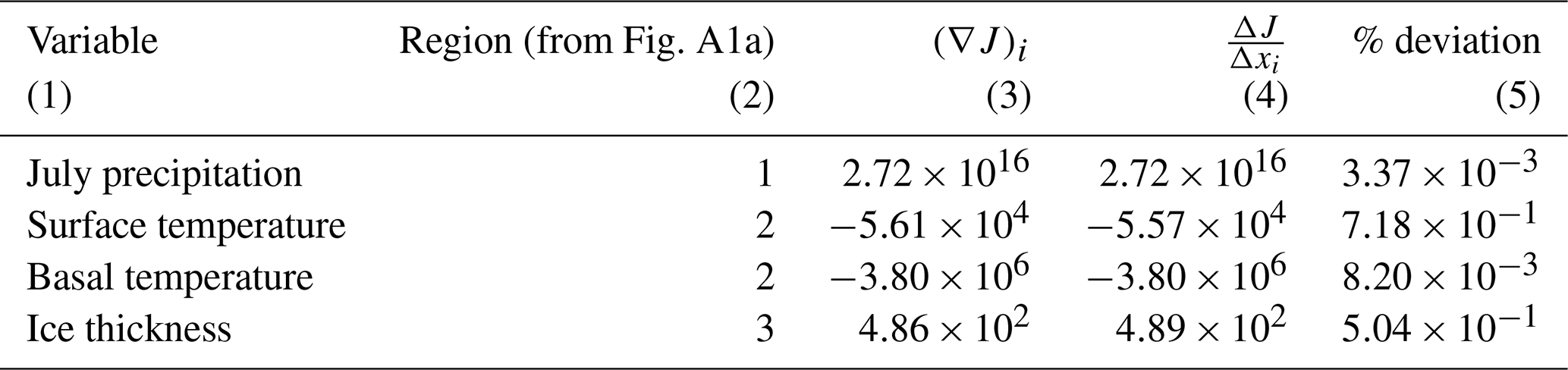
Figure A1Adjoint sensitivities, , for the Greenland Ice Sheet, where i is the control variable shown. Control variables are the (a) initial ice thickness (m2), (b) mean July precipitation (m2 yr), (c) surface temperature (m3 ∘C−1), and (d) basal temperature (m3 ∘C−1). Locations in (a) numbered 1–3 are compared to finite-difference values in Table A1.
Figure A1 shows the total Greenland Ice Sheet volume sensitivity to the initial condition of ice thickness and the boundary conditions in July (boreal summer) for precipitation as well as surface and basal temperatures. Table A1 shows that, in general, the Greenland simulation performs much better than the Antarctic simulation, with all of the percent deviations between adjoint values and finite-difference-based gradients less than 1 %. We attribute this to the lack of SSA dynamics involved and the accompanying use of an external solver library.
Interestingly, whereas in Antarctica the ice thickness sensitivities were almost entirely positive, substantial portions of the Greenland Ice Sheet lose volume when perturbed positively in ice thickness, a phenomenon previously inferred by Heimbach and Bugnion (2009) and thus a robust feature of SIA models. This could be due to the dynamic drawdown of glaciers that experience a sudden increase in driving stress due to the increase in ice thickness. The increase in driving stress leads to increases in velocity, which, when subjected to the land-ice-only mask for the SIA dynamics used in this setup of Greenland, results in the immediate cutoff of ice.
Sensitivity to precipitation, as in the case of Antarctica, is almost entirely positive and again dwarfs the other control variables tested here by many orders of magnitude. The overall larger magnitude of basal temperature sensitivities compared to surface temperatures is consistent with the Antarctic simulation. Completion of Greenland serial simulations on a Linux box (Intel Xeon CPU E5-2650 at 2.00 GHz) took 5, 10, and 140 min for horizontal resolutions of 40, 20, and 10 km, respectively. The results shown here are for 10 km resolution.
We made several modifications to SICOPOLIS to enable source transformation and differentiation via OpenAD.
The changes that were made enabled efficient AD in some cases and overcame some limitations of the AD tool used in
others. The modifications are guarded by C preprocessor (CPP) directive ALLOW_OPENAD and do
not affect the original behavior of SICOPOLIS in any way. Below, we discuss the noteworthy changes.
-
Data types. SICOPOLIS determines the number of bits for its data types at runtime through the calls
selected_int_kind()andkind(). Because OpenAD requires full knowledge of the types for static analysis, it does not support this behavior. We therefore determine the number of bits per type separately for the machine being used and specify the value directly in the code.
-
Unstructured code. The adjoint model of OpenAD reverses the control flow of the original code, including that of loops. It uses the following criteria to evaluate whether the loops are simple.
-
Loop variables are not updated within the loop
-
The loop condition does not use
.ne. -
The loop condition’s left-hand side consists only of the loop variable
-
The stride in the update expression is fixed
-
The stride is the right-hand side of the top level
.+or.-operator -
The loop body contains no index expression with variables that are modified within the loop body
SICOPOLIS contained several cases of statements injected to break out of loops that cause them not to be simple. To differentiate non-simple loops correctly, OpenAD stores which array indices are actually used per loop iteration. This approach causes significant memory usage and performance loss. Therefore, we removed the
exitstatements by rewriting the loop body to include a conditional statement that executes the loop only when the original loop would not exit. Restricting code to comply with “simple loops” is common in models subject to AD and is good coding practice in general, as it supports compiler optimization of loops.
-
-
Non-smoothness. Non-smoothness in the underlying mathematics of a model can be caused by the use of the absolute value, ceiling, and floor functions. Non-smooth models can be non-differentiable at a few or many points of the input space. Techniques such as piecewise linear differentiation and the absnormal form have been studied to differentiate non-smooth applications (Streubel et al., 2014). While SICOPOLIS employs all three functions, they are either used to index into lookup tables or used in portions not differentiated by OpenAD. Because OpenAD does not include
abs,ceiling, andflooras functions within its intrinsic library, we created custom subroutines of these functions to be differentiated.
-
The
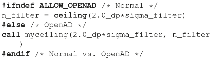
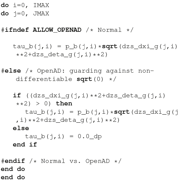
sqrtfunction. The derivative of is . When x=0.0, the result is a kink in the adjoint model and the appearance ofNaNin the adjoint computation. The intended behavior of the adjoint model is to treat the derivatives as 0.0. Therefore, wherever the functionsqrt()appears in SICOPOLIS, we use a conditional to check if the input tosqrt()is0.0, and in those cases we use0.0instead of callingsqrt().
-
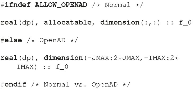
Array declaration and array assignments. SICOPOLIS uses dynamic memory allocation for some arrays in the code. Because the handling of dynamic memory and pointers by source transformation AD tools such as OpenAD remains a topic of active research, we replaced the dynamic allocation with static allocation.
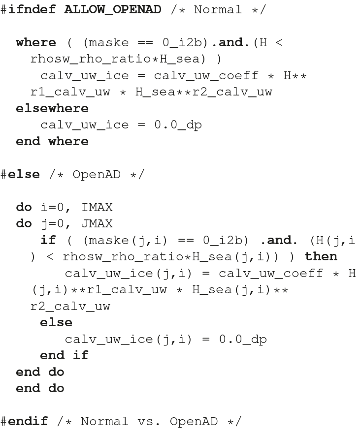
SICOPOLIS uses constructs such aswhereandelsewhereto elegantly assign values to array elements. Because OpenAD does not support these constructs, we rewrote them using loops andifstatements.
-
Intent of variables. SICOPOLIS passes the indices of two- and three-dimensional arrays as arguments with
intent(in)to subroutines that act upon particular portions of the array. When these variables are not the type of active variable (usuallyreal(dp)), their declarations must be changed tointent(inout). For variables that are active OpenAD changes the intent automatically.
-
Solvers. SICOPOLIS employs an array of solvers depending on the domain (e.g., Greenland versus Antarctica) or physics chosen by the user: a successive over-relaxation (SOR) solver, a tridiagonal solver, and (for Antarctic domains) the library of iterative solvers (LIS) for computing a system of linear equations:
To differentiate the above formulation efficiently, an AD tool must not naively differentiate through the solver code. OpenAD uses its
templatemechanism instead to encode the formulation below (Giles, 2008) to compute the adjoints and from using the original solver call:When SICOPOLIS uses the SOR solver for a system of linear equations wherein the matrix storage is in compressed sparse row (CSR) format, arrays are represented by
lgs_a_value(values),lgs_a_index(indices), andlgs_a_ptr(pointers). While the symbolic differentiation of the solver can be handled as above, the formation of the CSR representation requires us to change the type of the indices intoreal(dp)so that the indices are stored in the forward sweep for use in the reverse sweep.
-
Checkpointing. For adjoint models, the memory requirement to compute the adjoint information is proportional to the operation count of the model being differentiated. We found that the memory requirements of the adjoint model of SICOPOLIS for even small number of time steps will quickly exceed the available memory of most machines. Therefore, we implemented a binomial checkpointing scheme using the library
revolve(Griewank and Walther, 2000). This approach uses the recomputation of time steps in the original model to reduce the memory requirements of the adjoint model.
SICOPOLIS is free and open-source software available through a persistent Subversion repository that is hosted by the FusionForge system AWIForge of the Alfred Wegener Institute for Polar and Marine Research (AWI) in Bremerhaven, Germany (https://swrepo1.awi.de/, AWI FusionForge, 2020). Detailed instructions for obtaining and compiling the code are at http://www.sicopolis.net (SICOPOLIS.net, 2020). The adjoint generation capability of SICOPOLIS is a part of the main trunk of the current developmental version (5-dev). The development and tests were performed using SICOPOLIS v5-dev (revision 1414), tagged as SICOPOLIS-AD v1. It can be specifically downloaded at https://swrepo1.awi.de/svn/sicopolis/tags/ad-v1 (last access: 2 April 2020) (using “svn checkout” with “anonsvn” as the username and password). A snapshot non-revocable code archive of SICOPOLIS-AD v1 has been created at https://doi.org/10.5281/zenodo.3686393 (Logan et al., 2020).
The AD tool used to generate adjoint source code is OpenAD. A snapshot non-revocable code archive of OpenAD can be downloaded at https://doi.org/10.5281/zenodo.3361744 (Narayanan, 2019). Detailed instructions on how to download and build the tool are at https://www.mcs.anl.gov/OpenAD/ (last access: 2 April 2020). Technical details on how to set up, compile, and run reference configurations of SICOPOLIS-AD are documented in a quick-start manual (Logan et al., 2019), a version of which has also been placed in the SICOPOLIS-AD Zenodo archive.
LCL, SHKN, and PH developed the adjoint code of SICOPOLIS; RG originally developed SICOPOLIS, provided insight on the model results, and helped host the freely available version of the code.
The authors declare that they have no conflict of interest.
We thank Laurent Hascoët, Mauro Perego, and Lizz Ultee for their careful reviews, thoughtful comments, and valuable suggestions, which helped to improve the paper.
This research has been supported by the U.S. Department of Energy, Office of Science (grant no. DE-AC02-06CH11357 and SC0008060), the U.S. National Science Foundation (grant no. 1750035), the Japan Society for the Promotion of Science (KAKENHI grant nos. JP16H02224, JP17H06104 and JP17H06323), and the Japanese Ministry of Education, Culture, Sports, Science and Technology (MEXT) through the Arctic Challenge for Sustainability (ArCS) project (program grant number JPMXD1300000000).
This paper was edited by Alexander Robel and reviewed by Laurent Hascoet, Lizz Ultee, and one anonymous referee.
Arthern, R. J., Winebrenner, D. P., and Vaughan, D. G.: Antarctic snow accumulation mapped using polarization of 4.3-cm wavelength microwave emission, J. Geophys. Res.-Atmos., 111, D06107, https://doi.org/10.1029/2004JD005667, 2006. a
Aschwanden, A., Bueler, E., Khroulev, C., and Blatter, H.: An enthalpy formulation for glaciers and ice sheets, J. Glaciol., 58, 441–457, https://doi.org/10.3189/2012JoG11J088, 2012. a
AWI FusionForge: Alfred Wegener Institute for Polar and Marine Research FusionForge, available at: https://swrepo1.awi.de, last access: 6 April 2020. a
Balmaseda, M. A.: Editorial for Ocean Reanalysis Intercomparison Special Issue, Clim. Dynam., 49, 707–708, https://doi.org/10.1007/s00382-017-3813-8, 2017. a
Bamber, J. L., Layberry, R. L., and Gogenini, S. P.: A new ice thickness and bed data set for the Greenland ice sheet 1. Measurement, data reduction, and errors, J. Geophys. Res.-Atmos., 106, 33773–33780, https://doi.org/10.1029/2001JD900054, 2001. a
Bamber, J. L., Griggs, J. A., Hurkmans, R. T. W. L., Dowdeswell, J. A., Gogineni, S. P., Howat, I., Mouginot, J., Paden, J., Palmer, S., Rignot, E., and Steinhage, D.: A new bed elevation dataset for Greenland, The Cryosphere, 7, 499–510, https://doi.org/10.5194/tc-7-499-2013, 2013. a
Bernales, J., Rogozhina, I., Greve, R., and Thomas, M.: Comparison of hybrid schemes for the combination of shallow approximations in numerical simulations of the Antarctic Ice Sheet, The Cryosphere, 11, 247–265, https://doi.org/10.5194/tc-11-247-2017, 2017. a, b, c
Brinkerhoff, D. J. and Johnson, J. V.: Data assimilation and prognostic whole ice sheet modelling with the variationally derived, higher order, open source, and fully parallel ice sheet model VarGlaS, The Cryosphere, 7, 1161–1184, https://doi.org/10.5194/tc-7-1161-2013, 2013. a, b
Budd, W. F., Jenssen, D., and Smith, I. N.: A three-dimensional time-dependent model of the West Antarctic ice sheet, Ann. Glaciol., 5, 29–36, 1984. a
Cuffey, K. M. and Paterson, W. S. B.: The Physics of Glaciers, Elsevier, Amsterdam, The Netherlands, 4th Edn., 2010. a, b
Errico, R. M. and Vukicevic, T.: Sensitivity analysis using an adjoint of the PSU-NCAR mesoseale model, Mon. Weather Rev., 120, 1644–1660, https://doi.org/10.1175/1520-0493(1992)120<1644:SAUAAO>2.0.CO;2, 1992. a, b
Forget, G., Campin, J.-M., Heimbach, P., Hill, C. N., Ponte, R. M., and Wunsch, C.: ECCO version 4: an integrated framework for non-linear inverse modeling and global ocean state estimation, Geosci. Model Dev., 8, 3071–3104, https://doi.org/10.5194/gmd-8-3071-2015, 2015. a
Forth, S., Hovland, P., Phipps, E., Utke, J., and Walther, A. (Eds.): Recent Advances in Algorithmic Differentiation, Lecture Notes in Computational Science and Engineering, Springer Science & Business Media, Vol. 87, https://doi.org/10.1007/978-3-642-30023-3, 2012. a
Fortuin, J. P. F. and Oerlemans, J.: Parameterization of the annual surface temperature and mass balance of Antarctica, Ann. Glaciol., 14, 78–84, https://doi.org/10.3189/S0260305500008302, 1990. a
Fretwell, P., Pritchard, H. D., Vaughan, D. G., Bamber, J. L., Barrand, N. E., Bell, R., Bianchi, C., Bingham, R. G., Blankenship, D. D., Casassa, G., Catania, G., Callens, D., Conway, H., Cook, A. J., Corr, H. F. J., Damaske, D., Damm, V., Ferraccioli, F., Forsberg, R., Fujita, S., Gim, Y., Gogineni, P., Griggs, J. A., Hindmarsh, R. C. A., Holmlund, P., Holt, J. W., Jacobel, R. W., Jenkins, A., Jokat, W., Jordan, T., King, E. C., Kohler, J., Krabill, W., Riger-Kusk, M., Langley, K. A., Leitchenkov, G., Leuschen, C., Luyendyk, B. P., Matsuoka, K., Mouginot, J., Nitsche, F. O., Nogi, Y., Nost, O. A., Popov, S. V., Rignot, E., Rippin, D. M., Rivera, A., Roberts, J., Ross, N., Siegert, M. J., Smith, A. M., Steinhage, D., Studinger, M., Sun, B., Tinto, B. K., Welch, B. C., Wilson, D., Young, D. A., Xiangbin, C., and Zirizzotti, A.: Bedmap2: improved ice bed, surface and thickness datasets for Antarctica, The Cryosphere, 7, 375–393, https://doi.org/10.5194/tc-7-375-2013, 2013. a
Gelb, A. (Ed.): Applied Optimal Estimation, The MIT Press, 1974. a
Giering, R., Kaminski, T., and Slawig, T.: Generating efficient derivative code with TAF: Adjoint and tangent linear Euler flow around an airfoil, Future Gener. Comp. Sy., 21, 1345–1355, https://doi.org/10.1016/j.future.2004.11.003, 2005. a, b
Giles, M. B.: Collected Matrix Derivative Results for Forward and Reverse Mode Algorithmic Differentiation, in: Advances in Automatic Differentiation, edited by: Bischof, C. H., Bücker, H. M., Hovland, P., Naumann, U., and Utke, J., Springer Berlin Heidelberg, Berlin, Heidelberg, 35–44, 2008. a
Gillet-Chaulet, F., Gagliardini, O., Seddik, H., Nodet, M., Durand, G., Ritz, C., Zwinger, T., Greve, R., and Vaughan, D. G.: Greenland ice sheet contribution to sea-level rise from a new-generation ice-sheet model, The Cryosphere, 6, 1561–1576, https://doi.org/10.5194/tc-6-1561-2012, 2012. a, b
Glasser, N. F. and Scambos, T. A.: A structural glaciological analysis of the 2002 Larsen B ice-shelf collapse, J. Glaciol., 54, 3–16, https://doi.org/10.3189/002214308784409017, 2008. a
Glen, J. W.: The creep of polycrystalline ice, P. R. Soc. A, 228, 519–538, https://doi.org/10.1098/rspa.1955.0066, 1955. a
Goelzer, H., Nowicki, S., Edwards, T., Beckley, M., Abe-Ouchi, A., Aschwanden, A., Calov, R., Gagliardini, O., Gillet-Chaulet, F., Golledge, N. R., Gregory, J., Greve, R., Humbert, A., Huybrechts, P., Kennedy, J. H., Larour, E., Lipscomb, W. H., Le clec'h, S., Lee, V., Morlighem, M., Pattyn, F., Payne, A. J., Rodehacke, C., Rückamp, M., Saito, F., Schlegel, N., Seroussi, H., Shepherd, A., Sun, S., van de Wal, R., and Ziemen, F. A.: Design and results of the ice sheet model initialisation experiments initMIP-Greenland: an ISMIP6 intercomparison, The Cryosphere, 12, 1433–1460, https://doi.org/10.5194/tc-12-1433-2018, 2018. a, b
Goldberg, D. N. and Heimbach, P.: Parameter and state estimation with a time-dependent adjoint marine ice sheet model, The Cryosphere, 7, 1659–1678, https://doi.org/10.5194/tc-7-1659-2013, 2013. a, b, c
Goldberg, D. N. and Sergienko, O. V.: Data assimilation using a hybrid ice flow model, The Cryosphere, 5, 315–327, https://doi.org/10.5194/tc-5-315-2011, 2011. a, b
Goldberg, D. N., Heimbach, P., Joughin, I., and Smith, B.: Committed retreat of Smith, Pope, and Kohler Glaciers over the next 30 years inferred by transient model calibration, The Cryosphere, 9, 2429–2446, https://doi.org/10.5194/tc-9-2429-2015, 2015. a
Goldberg, D. N., Narayanan, S. H. K., Hascoet, L., and Utke, J.: An optimized treatment for algorithmic differentiation of an important glaciological fixed-point problem, Geosci. Model Dev., 9, 1891–1904, https://doi.org/10.5194/gmd-9-1891-2016, 2016. a, b
Greve, R.: A continuum-mechanical formulation for shallow polythermal ice sheets, Philos. T. R. Soc. A, 355, 921–974, https://doi.org/10.1098/rsta.1997.0050, 1997. a
Greve, R.: Geothermal heat flux distribution for the Greenland ice sheet, derived by combining a global representation and information from deep ice cores, Polar Data J., 3, 22–36, https://doi.org/10.20575/00000006, 2019. a
Greve, R. and Blatter, H.: Dynamics of Ice Sheets and Glaciers, Springer, Berlin, Germany, https://doi.org/10.1007/978-3-642-03415-2, 2009. a, b
Greve, R. and Blatter, H.: Comparison of thermodynamics solvers in the polythermal ice sheet model SICOPOLIS, Polar Sci., 10, 11–23, https://doi.org/10.1016/j.polar.2015.12.004, 2016. a, b
Greve, R. and Calov, R.: Comparison of numerical schemes for the solution of the ice-thickness equation in a dynamic/thermodynamic ice-sheet model, J. Comput. Phys., 179, 649–664, https://doi.org/10.1006/jcph.2002.7081, 2002. a
Griewank, A. and Walther, A.: Algorithm 799: revolve: an implementation of checkpointing for the reverse or adjoint mode of computational differentiation, ACM T. Math. Software, 26, 19–45, https://doi.org/10.1145/347837.347846, 2000. a
Griewank, A. and Walther, A.: Evaluating Derivatives: Principles and Techniques of Algorithmic Differentiation, Other Titles in Applied Mathematics, Society for Industrial and Applied Mathematics, Philadelphia, PA, US, 2nd Edn., https://doi.org/10.1137/1.9780898717761, 2008. a
Hascoët, L. and Morlighem, M.: Source-to-source adjoint Algorithmic Differentiation of an ice sheet model written in C, Optim. Method. Softw., 33, 1–8, https://doi.org/10.1080/10556788.2017.1396600, 2018. a
Hascoët, L. and Utke, J.: Programming language features, usage patterns, and the efficiency of generated adjoint code, Optim. Method. Softw., 31, 885–903, https://doi.org/10.1080/10556788.2016.1146269, 2016. a
Heimbach, P. and Bugnion, V.: Greenland ice-sheet volume sensitivity to basal, surface and initial conditions derived from an adjoint model, Ann. Glaciol., 50, 67–80, https://doi.org/10.3189/172756409789624256, 2009. a, b, c, d, e, f, g, h
Heimbach, P., Hill, C., and Giering, R.: Automatic generation of efficient adjoint code for a parallel Navier-Stokes solver, in: Computational Science – ICCS 2002, edited by: Sloot, P. M. A., Hoekstra, A. G., Tan, C. J. K., and Dongarra, J. J., Springer, Berlin, Heidelberg, 1019–1028, 2002. a
Heimbach, P., Hill, C., and Giering, R.: An efficient exact adjoint of the parallel MIT general circulation model, generated via automatic differentiation, Future Gener. Comp. Sy., 21, 1356–1371, https://doi.org/10.1016/j.future.2004.11.010, 2005. a, b
Hoffman, M. J., Perego, M., Price, S. F., Lipscomb, W. H., Zhang, T., Jacobsen, D., Tezaur, I., Salinger, A. G., Tuminaro, R., and Bertagna, L.: MPAS-Albany Land Ice (MALI): a variable-resolution ice sheet model for Earth system modeling using Voronoi grids, Geosci. Model Dev., 11, 3747–3780, https://doi.org/10.5194/gmd-11-3747-2018, 2018. a
Hutter, K.: Theoretical Glaciology; Material Science of Ice and the Mechanics of Glaciers and Ice Sheets, D. Reidel Publishing Company, Dordrecht, The Netherlands, 1983. a
Isaac, T., Stadler, G., and Ghattas, O.: Solution of nonlinear Stokes equations discretized by high-order finite elements on nonconforming and anisotropic meshes, with application to ice sheet dynamics, SIAM J. Sci. Comput., 37, B804–B833, https://doi.org/10.1137/140974407, 2015. a, b
Joughin, I., Tulaczyk, S., Bamber, J. L., Blankenship, D., Holt, J. W., Scambos, T., and Vaughan, D. G.: Basal conditions for Pine Island and Thwaites Glaciers, West Antarctica, determined using satellite and airborne data, J. Glaciol., 55, 245–257, https://doi.org/10.3189/002214309788608705, 2009. a
Khazendar, A., Rignot, E., and Larour, E.: Larsen B Ice Shelf rheology preceding its disintegration inferred by a control method, Geophys. Res. Lett., 34, L19503, https://doi.org/10.1029/2007GL030980, 2007. a
Larour, E., Rignot, E., Joughin, I., and Aubry, D.: Rheology of the Ronne Ice Shelf, Antarctica, inferred from satellite radar interferometry data using an inverse control method, Geophys. Res. Lett., 32, L05503, https://doi.org/10.1029/2004GL021693, 2005. a
Larour, E., Utke, J., Csatho, B., Schenk, A., Seroussi, H., Morlighem, M., Rignot, E., Schlegel, N., and Khazendar, A.: Inferred basal friction and surface mass balance of the Northeast Greenland Ice Stream using data assimilation of ICESat (Ice Cloud and land Elevation Satellite) surface altimetry and ISSM (Ice Sheet System Model), The Cryosphere, 8, 2335–2351, https://doi.org/10.5194/tc-8-2335-2014, 2014. a, b
Le Brocq, A. M., Payne, A. J., and Vieli, A.: An improved Antarctic dataset for high resolution numerical ice sheet models (ALBMAP v1), Earth Syst. Sci. Data, 2, 247–260, https://doi.org/10.5194/essd-2-247-2010, 2010. a
Liao, H.-J., Liu, J.-G., Wang, L., and Xiang, T.: Differentiable programming tensor networks, Phys. Rev. X, 9, 031041, https://doi.org/10.1103/PhysRevX.9.031041, 2019. a
Lliboutry, L. and Duval, P.: Various isotropic and anisotropic ices found in glaciers and polar ice caps and their corresponding rheologies, Ann. Geophys., 3, 207–224, 1985. a
Logan, L. C., Narayanan, S. H. K., Greve, R., and Heimbach, P.: SICOPOLIS-AD: Quick-Start Manual, Technical Report ANL/MCS-TM-382 Rev 0.10, Argonne National Laboratory, ANL, Argonne, IL, https://doi.org/10.2172/1499025, 2019. a, b, c
Logan, L. C., Narayanan, S. H. K., Greve, R., and Heimbach, P.: SICOPOLIS-AD v1 (Version 1), Zenodo, https://doi.org/10.5281/zenodo.3686393, 2020. a
MacAyeal, D. R.: Ice-shelf response to ice-stream discharge fluctuations: III. The effects of ice-stream imbalance on the Ross Ice Shelf, Antarctica, J. Glaciol., 35, 38–42, https://doi.org/10.3189/002214389793701545, 1989. a
MacAyeal, D. R., Firestone, J., and Waddington, E.: Paleothermometry by control methods, J. Glaciol., 37, 326–338, https://doi.org/10.3189/S0022143000005761, 1991. a
Marotzke, J., Giering, R., Zhang, K. Q., Stammer, D., Hill, C., and Lee, T.: Construction of the adjoint MIT ocean general circulation model and application to Atlantic heat transport variability, J. Geophys. Res.-Oceans, 104, 29529–29547, https://doi.org/10.1029/1999JC900236, 1999. a
Marsiat, I.: Simulation of the northern hemisphere continental ice sheets over the last glacial-interglacial cycle: Experiments with a latitude-longitude vertically integrated ice sheet model coupled to zonally averaged climate model, Paleoclimates, 1, 59–98, 1994. a
Meehl, G. A., Moss, R., Taylor, K. E., Eyring, V., Stouffer, R. J., Bony, S., and Stevens, B.: Climate model intercomparisons: preparing for the next phase, Eos T. Am. Geophys. Un., 95, 77–78, https://doi.org/10.1002/2014EO090001, 2014. a
Morland, L. W.: Thermomechanical balances of ice sheet flows, Geophys. Astro. Fluid, 29, 237–266, https://doi.org/10.1080/03091928408248191, 1984. a
Morland, L. W.: Unconfined ice-shelf flow, in: Dynamics of the West Antarctic Ice Sheet, edited by: van der Veen, C. J. and Oerlemans, J., D. Reidel Publishing Company, Dordrecht, The Netherlands, 99–116, 1987. a
Morlighem, M., Rignot, E., Seroussi, H., Larour, E., Ben Dhia, H., and Aubry, D.: Spatial patterns of basal drag inferred using control methods from a full-Stokes and simpler models for Pine Island Glacier, West Antarctica, Geophys. Res. Lett., 37, L14502, https://doi.org/10.1029/2010GL043853, 2010. a
Morlighem, M., Seroussi, H., Larour, E., and Rignot, E.: Inversion of basal friction in Antarctica using exact and incomplete adjoints of a higher-order model, J. Geophys. Res.-Earth, 118, 1746–1753, https://doi.org/10.1002/jgrf.20125, 2013. a, b
Mosbeux, C., Gillet-Chaulet, F., and Gagliardini, O.: Comparison of adjoint and nudging methods to initialise ice sheet model basal conditions, Geosci. Model Dev., 9, 2549–2562, https://doi.org/10.5194/gmd-9-2549-2016, 2016. a
Narayanan, S. H. K.: sriharikrishna/OpenAD: SICOPOLIS-AD v1 (Version SICOPOLIS-AD), Zenodo, https://doi.org/10.5281/zenodo.3361744, 2019. a
Naumann, U.: The Art of Differentiating Computer Programs: An Introduction to Algorithmic Differentiation, Software, Environments and Tools, 333 pp., https://doi.org/10.1137/1.9781611972078, SIAM Press, 2012. a
Perego, M., Price, S., and Stadler, G.: Optimal initial conditions for coupling ice sheet models to Earth system models, J. Geophys. Res.-Earth, 119, 1894–1917, https://doi.org/10.1002/2014JF003181, 2014. a
Petra, N., Zhu, H., Stadler, G., Hughes, T. J. R., and Ghattas, O.: An inexact Gauss-Newton method for inversion of basal sliding and rheology parameters in a nonlinear Stokes ice sheet model, J. Glaciol., 58, 889–903, https://doi.org/10.3189/2012JoG11J182, 2012. a
Ritz, C.: EISMINT intercomparison experiment: comparison of existing Greenland models, Laboratoire de Glaciologie et de Géophysique de l’Environnement, Saint Martin d’Hères, France, 105 1997. a
Robinson, A., Calov, R., and Ganopolski, A.: An efficient regional energy-moisture balance model for simulation of the Greenland Ice Sheet response to climate change, The Cryosphere, 4, 129–144, https://doi.org/10.5194/tc-4-129-2010, 2010. a
Rückamp, M., Greve, R., and Humbert, A.: Comparative simulations of the evolution of the Greenland ice sheet under simplified Paris Agreement scenarios with the models SICOPOLIS and ISSM, Polar Sci., 21, 14–25, https://doi.org/10.1016/j.polar.2018.12.003, 2019. a
Seroussi, H., Nowicki, S., Simon, E., Abe-Ouchi, A., Albrecht, T., Brondex, J., Cornford, S., Dumas, C., Gillet-Chaulet, F., Goelzer, H., Golledge, N. R., Gregory, J. M., Greve, R., Hoffman, M. J., Humbert, A., Huybrechts, P., Kleiner, T., Larour, E., Leguy, G., Lipscomb, W. H., Lowry, D., Mengel, M., Morlighem, M., Pattyn, F., Payne, A. J., Pollard, D., Price, S. F., Quiquet, A., Reerink, T. J., Reese, R., Rodehacke, C. B., Schlegel, N.-J., Shepherd, A., Sun, S., Sutter, J., Van Breedam, J., van de Wal, R. S. W., Winkelmann, R., and Zhang, T.: initMIP-Antarctica: an ice sheet model initialization experiment of ISMIP6, The Cryosphere, 13, 1441–1471, https://doi.org/10.5194/tc-13-1441-2019, 2019. a, b
SICOPOLIS.net: Ice sheet model SICOPOLIS, homepage, available at: http://www.sicopolis.net, last access: 6 April 2020. a
Streubel, T., Griewank, A., Radons, M., and Bernt, J.-U.: Representation and Analysis of Piecewise Linear Functions in Abs-Normal Form, in: System Modeling and Optimization, edited by: Pötzsche C., Heuberger C., Kaltenbacher B., Rendl F., CSMO 2013, IFIP Advances in Information and Communication Technology, 443, 327–336, https://doi.org/10.1007/978-3-662-45504-3_32, Springer, Berlin, Heidelberg, 1997. a
Talagrand, O. and Courtier, P.: Variational assimilation of meteorological observations with the adjoint vorticity equation. I: Theory, Q. J. Roy. Meteor. Soc., 113, 1311–1328, https://doi.org/10.1002/qj.49711347812, 1987. a
Thacker, W. C. and Long, R. B.: Fitting dynamics to data, J. Geophys. Res.-Oceans, 93, 1227–1240, https://doi.org/10.1029/JC093iC02p01227, 1988. a
Uppala, S. M., Kållberg, P. W., Simmons, A. J., Andrae, U., Da Costa Bechtold, V., Fiorino, M., Gibson, J. K., Haseler, J., Hernandez, A., Kelly, G. A., Li, X., Onogi, K., Saarinen, S., Sokka, N., Allan, R. P., Andersson, E., Arpe, K., Balmaseda, M. A., Beljaars, A. C. M., Van De Berg, L., Bidlot, J., Bormann, N., Caires, S., Chevallier, F., Dethof, A., Dragosavac, M., Fisher, M., Fuentes, M., Hagemann, S., Hólm, E., Hoskins, B. J., Isaksen, L., Janssen, P. A. E. M., Jenne, R., Mcnally, A. P., Mahfouf, J.-F., Morcrette, J.-J., Rayner, N. A., Saunders, R. W., Simon, P., Sterl, A., Trenberth, K. E., Untch, A., Vasiljevic, D., Viterbo, P., and Woollen, J.: The ERA-40 re-analysis, Q. J. Roy. Meteor. Soc., 131, 2961–3012, https://doi.org/10.1256/qj.04.176, 2005. a
Utke, J., Naumann, U., Fagan, M., Tallent, N., Strout, M., Heimbach, P., Hill, C., Ozyurt, D., and Wunsch, C.: OpenAD/F: A modular open source tool for automatic differentiation of Fortran codes, ACM T. Math. Softw., 34, 18, https://doi.org/10.1145/1377596.1377598, 2008. a
Vieli, A. and Payne, A. J.: Application of control methods for modelling the flow of Pine Island Glacier, West Antarctica, Ann. Glaciol., 36, 197–204, https://doi.org/10.3189/172756403781816338, 2003. a
Waddington, E. D., Neumann, T. A., Koutnik, M. R., Marshall, H.-P., and Morse, D. L.: Inference of accumulation-rate patterns from deep layers in glaciers and ice sheets, J. Glaciol., 53, 694–712, https://doi.org/10.3189/002214307784409351, 2007. a
Weertman, J.: The theory of glacier sliding, J. Glaciol., 5, 287–303, https://doi.org/10.3189/S0022143000029038, 1964. a
Weis, M., Greve, R., and Hutter, K.: Theory of shallow ice shelves, Continuum Mech. Therm., 11, 15–50, https://doi.org/10.1007/s001610050102, 1999. a
Wunsch, C. and Heimbach, P.: Practical global oceanic state estimation, Physica D, 230, 197–208, https://doi.org/10.1016/j.physd.2006.09.040, 2007. a, b, c
- Abstract
- Introduction
- Model description
- Example application: Antarctic Ice Sheet volume sensitivities
- Discussion
- Conclusions
- Appendix A: Greenland ice volume sensitivities
- Appendix B: Modifying SICOPOLIS
- Code availability
- Author contributions
- Competing interests
- Acknowledgements
- Financial support
- Review statement
- References