2.1 BESM-OA2.5

BESM-OA2.5 is the result of coupling the Center for Weather Forecast and Climate Studies (CPTEC/INPE) Brazilian Atmospheric Model (BAM; Figueroa et al., 2016) and the Geophysical Fluid Dynamics Laboratory (GFDL) Modular Ocean Model version 4p1 (Griffies et al., 2004) via the Flexible Modular System (FMS) (also from GFDL). The dynamical core and physical parameterizations of the atmospheric component of BESM-OA2.5 are the same as those discussed in Veiga et al. (2019). BAM is a hydrostatic model, with its dynamical core based on the spectral transform method, which employs global spherical harmonic basis functions. The Eulerian advection scheme option is used in this study, with a two-time-level semi-Lagrangian scheme for the transport of moisture and microphysics prognostic variables, which are carried out completely within the model grid space. Simplified fast physical parameterizations are used here to increase the computational efficiency of long integrations, thus resulting in a decreased computational demand compared with that required by the operational Numerical Weather Prediction (NWP) model. A summary of the main differences in the physical parameterizations between BAM (as used in this paper) and the BAM NWP operational model is provided in Table 1. The dynamical equations in BAM are discretized following a spectral transform with horizontal resolution truncated at triangular wavenumber 62 (an equivalent grid size of approximately 1.875^∘) and 28 layers unevenly spaced in the vertical sigma coordinate with the top level at approximately 2.73 hPa. The oceanic component uses a tripolar grid at a horizontal resolution of 1^∘ in longitude, and in the latitudinal direction the grid spacing is 1∕4^∘ between 10^∘ S and 10^∘ N, decreasing uniformly to 1^∘ at 45^∘ and to 2^∘ at 90^∘ in both hemispheres. The ocean grid has 50 vertical levels with a 10 m resolution in the upper 220 m, decreasing gradually to approximately 370 m at deeper levels.

Table 1Atmospheric physical parameterizations used in BAM (Figueroa et al., 2016) BESM-OA2.5.

Download Print Version | Download XLSX

Veiga et al. (2019) showed that BESM-OA2.5 can capture the general mean climate state; however, substantial biases appeared in the simulation associated with a double Intertropical Convergence Zone (ITCZ) over the Pacific and Atlantic oceans and regional biases in the precipitation over the Amazon and Indian regions. BESM-OA2.5 can also reproduce the most important large-scale interannual and decadal climate variability patterns. The Atlantic Meridional Mode (AMM) (Nobre and Shukla, 1996) is well simulated by the model in terms of its spatial pattern and temporal variability, whereas this mode is poorly represented in most CMIP5 models (IPCC, 2013; Liu et al., 2013; Richter et al., 2014; Amaya et al., 2017). The maximum strength of the Atlantic Meridional Overturning Circulation (AMOC) represented by BESM-OA2.5 is 14 Sv, which is lower than the value determined within the RAPID project (17 Sv; McCarthy et al., 2015) but in the range of the observed root mean square variability, and this value is comparable to the ensemble AMOC simulated by the CMIP5 models. Moreover, the spatial structures of both the North Atlantic Oscillation (NAO) and the Pacific Decadal Oscillation (PDO) variability are well captured (Veiga et al., 2019).

2.2 Comparison to a previous model version

The recently developed BESM-OA2.5 is an advancement of BESM-OA2.3, which was presented by Nobre et al. (2013). The main differences between BESM-OA2.5 and the previous version (BESM-OA2.3) lie in the atmospheric model and how some surface layer variables are estimated. The total energy balance at the TOA is better represented in BESM-OA2.5 than in BESM-OA2.3, with a reduced global mean bias of approximately −4 W m⁻² compared with −20 W m⁻² for the latter. It should be noted that BESM-OA2.5 has a new set of parameterizations, mainly related to an improved representation of microphysical processes. For instance, the precipitation in the previous model was parameterized only in terms of the large-scale condensation. Moreover, BESM-OA2.5 underwent improvements in the representation of wind, humidity, and temperature in the surface layer with the use of the similarity functions method presented by Jiménez et al. (2012). Based on Monin–Obukhov theory, the wind (u_10 m), humidity (q_2 m), and temperature (θ_2 m) are estimated from the values of the first atmospheric model level and the surface, as described in Eqs. (24), (25), and (26) of Jiménez et al. (2012). Furthermore, the similarity functions ψ_m and ψ_h depend on the stability regimes (Businger et al., 1971). For BESM-OA2.5, those regimes are associated with stable ($\mathit{\zeta }/L>\mathrm{0}$) and unstable ($\mathit{\zeta }/L\le \mathrm{0}$) conditions (Arya, 1988). These diagnostic variables are important for BESM because they are used in the ocean–atmosphere coupling strategy.

Both versions reproduce the main climate variability, particularly over the Atlantic, such as the AMOC and the AMM, but simulate a weak El Niño–Southern Oscillation (ENSO) interannual variability over the equatorial Pacific (Nobre et al., 2013; Veiga et al., 2019). Concerning the general mean present-day climate state, BESM-OA2.5 shows improvements in reproducing the Intertropical Convergence Zone (ITCZ), and it reduces both the global precipitation root mean square error (RMSE) and the sea surface temperature (SST) RMSE compared with those modeled by BESM-OA2.3.

Global simulations that were 1 year long and 6-hourly outputs were performed with BAM configured with surface layer schemes based on Arya (1988) and Jiménez et al. (2012), here called BAM-Arya (the original scheme) and BAM-Jimenez (the new scheme), respectively. The normalized RMSE was computed with respect to the reanalysis NCEP-DOE (National Centers for Environmental Prediction – Department of Energy) version 2 (Kanamitsu et al., 2002). The normalized RMSE of the wind at 10 m and the temperature and humidity at 2 m for the two surface layer schemes was investigated. Consistent improvements of BAM-Jimenez relative to BAM-Arya were noted in all three variables over the oceanic regions. The normalized RMSE analysis over the continents yielded less consistent results, with an improved BAM-Jimenez representation of both winds and temperature but with an inferior representation of the humidity field (figures not shown).

3.1 Experimental design

For this study, climate simulations were performed using BESM-OA2.5 (hereinafter BESM) for the piControl (preindustrial control scenario, run for 300 years with atmospheric CO₂ concentration invariant at 274 ppmv) and abrupt4xCO2 (run for 150 years after the abrupt quadrupling of atmospheric CO₂ at year 151 of the piControl simulation) scenarios; therefore, both experiments were run in parallel for 150 years. These two scenarios are commonly employed in CMIP5 studies for climate sensitivity assessment (Taylor et al., 2012; Eyring et al., 2016). Climate change is evaluated as the difference between the abrupt4xCO2 and piControl experiments. In addition, BESM's results were compared with a selection of 25 CMIP5 models listed in Table 2. All models, including BESM, were interpolated at 2.5^∘ × 2.5^∘ longitude–latitude horizontal resolution. All CMIP5 model data are available from the Earth System Grid Federation (ESGF).

Table 2Models belonging to the CMIP5 ensemble used in this study.

Download Print Version | Download XLSX

3.2 Climate change sensitivity estimates

Here we estimate the climate feedback with two different methods using either a regression according to Gregory et al. (2004) or radiative kernels (Soden et al., 2004, 2008). The Gregory method is more straightforward computationally; however, it returns only a global mean value. Moreover, the ECS can be estimated with this method. On the other hand, it is possible to obtain the seasonal feedback for every latitude–longitude point with the radiative kernel method; furthermore, the feedback can be decomposed into different processes.

3.3 Changes in the atmospheric circulation and precipitation

Monthly mean climatologies were computed for the last 30 years of the piControl and abrupt4xCO2 runs, and the projected climate response to CO₂ increase was evaluated from the difference between these abrupt4xCO2 and piControl monthly mean climatologies. The statistical significance of this difference was calculated based on the Student's t test with a significance level of 90 %. Furthermore, to evaluate how similar two spatial patterns are, we used the spatial inner product calculated as $\sum (A_i\cdot B_i)/\left(\right|A|\cdot |B\left|\right)$, where A and B are the 2-D variables and i is the spatial index related to their latitude–longitude coordinates.

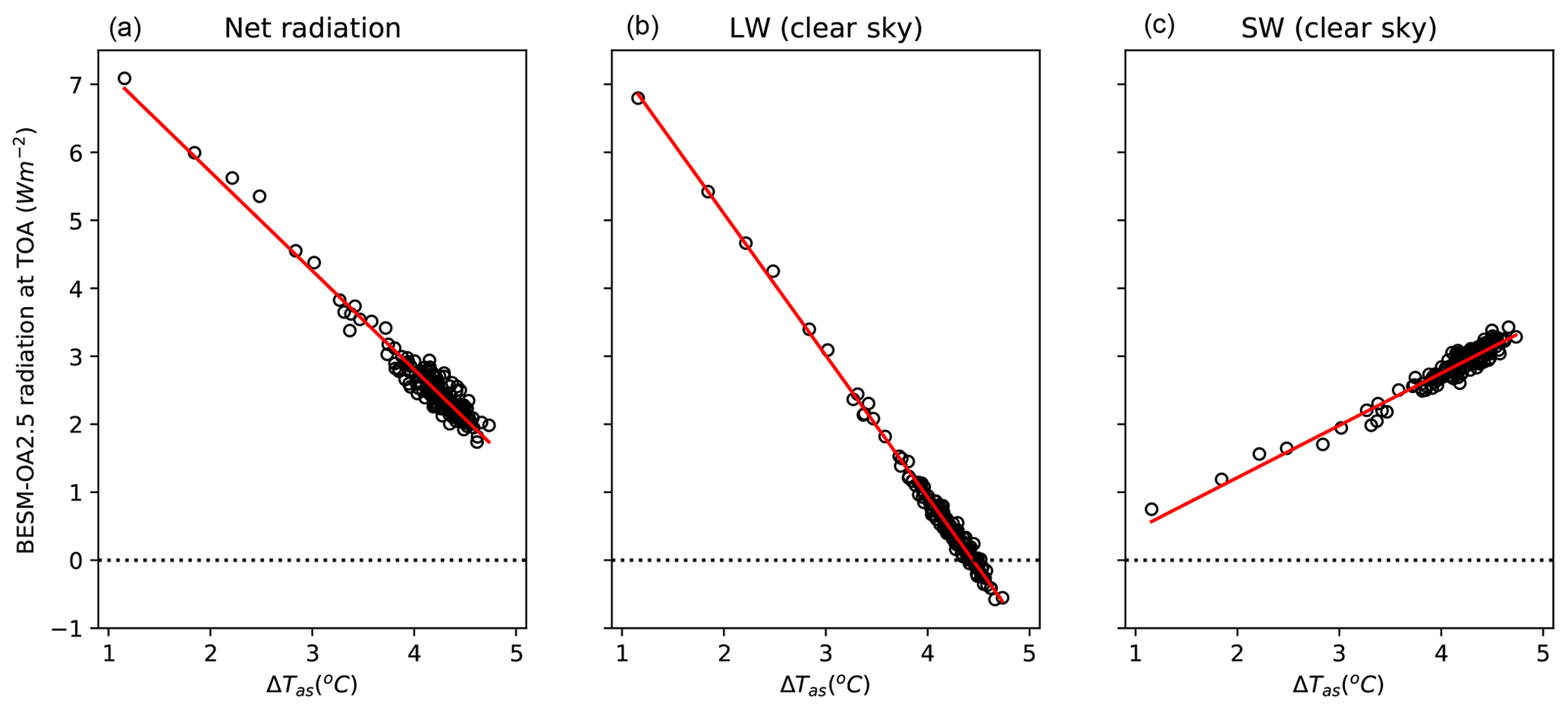
Figure 1Annual global mean linear regression between $\mathrm{\Delta }{\stackrel{\mathrm{‾}}{T}}_{\mathrm{as}}$ and (a) net radiation, (b) $\mathrm{\Delta }{\stackrel{\mathrm{‾}}{T}}_{\mathrm{as}}$ and ΔLW (clear sky), and (c) $\mathrm{\Delta }{\stackrel{\mathrm{‾}}{T}}_{\mathrm{as}}$ and ΔSW (clear sky) for BESM-OA2.5.

Download

4.1 G, λ, ΔCRE, and ECS estimated via the Gregory method

Figure 1 shows the linear regressions of ΔR , ΔLW (clear sky), and ΔSW (clear sky) against $\mathrm{\Delta }{\stackrel{\mathrm{‾}}{T}}_{\mathrm{as}}$ from BESM. The linear regressions based on all-sky radiative flux are used to estimate ECS, G, and λ, while the regressions based on clear-sky data are used to obtain ΔCRE (as mentioned in the previous section). BESM features G=8.62 W m⁻², $\mathit{\lambda }=-\mathrm{1.45}$ W m⁻² K⁻¹, $\mathrm{\Delta }\mathrm{CRE}=-\mathrm{0.13}$ W m⁻² K⁻¹, and ECS=2.96 K.

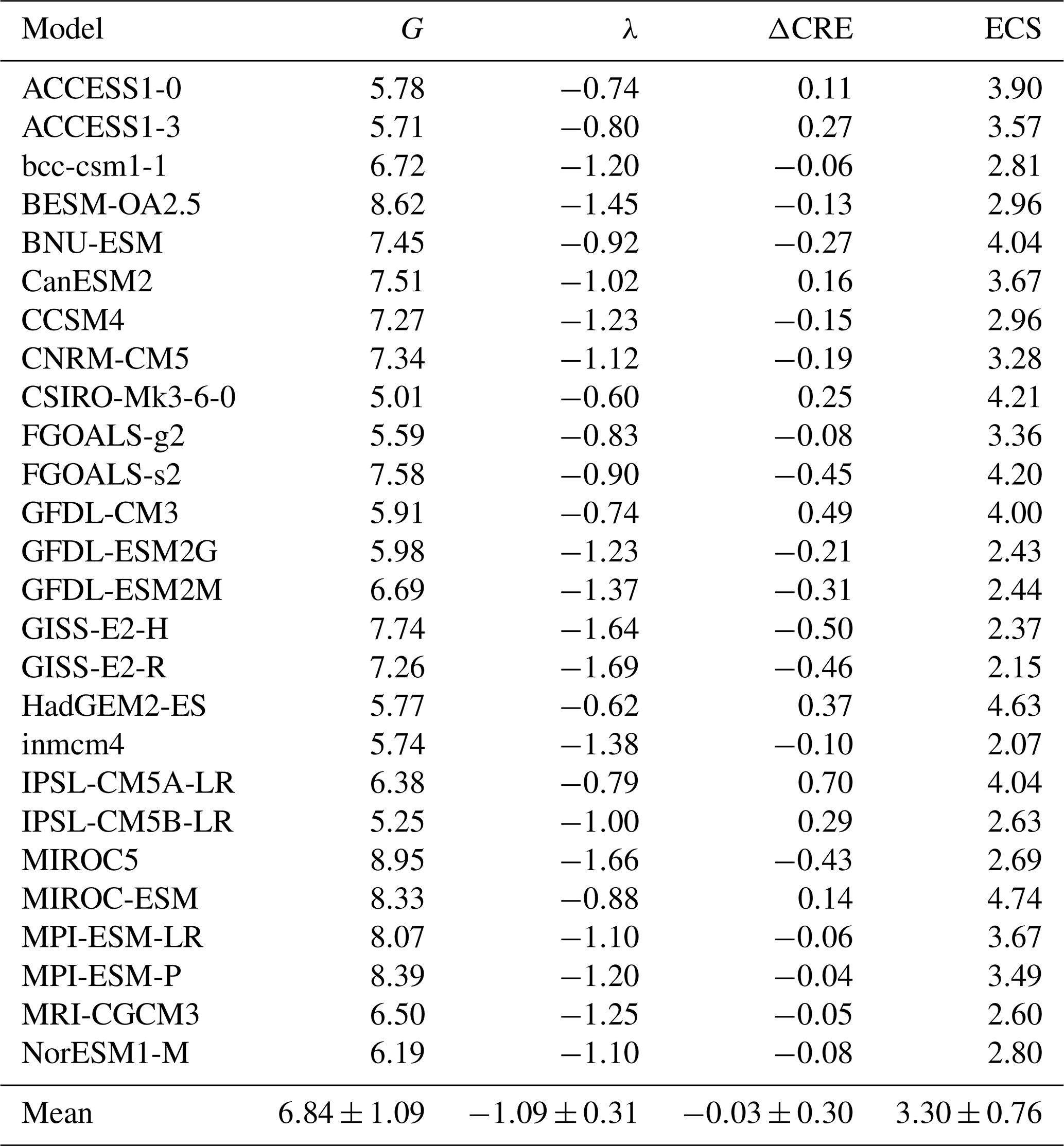
The parameters G, λ, ΔCRE, and ECS as computed for all models are shown in Table 3. The climate sensitivities of the 26 CMIP5 coupled models (including BESM-OA2.5) were compiled in an extension of the previous work by Andrews et al. (2012), who evaluated 15 CMIP5 coupled models. In the present work, we added the following models: ACCESS1-0, ACCESS1-3, bcc-csm1-1, BESM-OA2.5, BNU-ESM, CCSM4, FGOALS-g2, FGOALS-s2, GISS-E2-H, GISS-E2-R, and inmcm4. In Andrews et al. (2012) the ECS ranges from 2.07 to 4.74 K for the 15 models analyzed there, which is largely confirmed by our analysis. The small differences can possibly be attributed to the interpolation of the data. G and λ vary from 5.01 to 8.95 W m⁻² and from −1.66 to −0.60 W m⁻² K⁻¹, respectively. The inter-model spread in G among the models is due to differences in the radiative codes used and the rapid adjustment processes in the troposphere and at the surface (Collins et al., 2006; Gregory and Webb, 2008; Andrews and Forster, 2008). The spread in the ECS is more robustly influenced by λ than by G (Fig. 2), as was also suggested by Andrews et al. (2012). The correlation coefficient between the ECS and λ is −0.82, which is significant at a 1 % significance level (Fig. 2b). On the other hand, the correlation between the ECS and G is −0.01, which is not statistically significant (Fig. 2a). Thus, inter-model variation in the balance of feedbacks explains the dispersion in the ECS better than the initial radiative imbalance triggered by the CO₂ increase (related to G). Although BESM yielded one of the highest G values among all of the CMIP5 models, it showed a warming response to CO₂ doubling that is well within the range of 3.30±0.76 K as presented by the ensemble models.

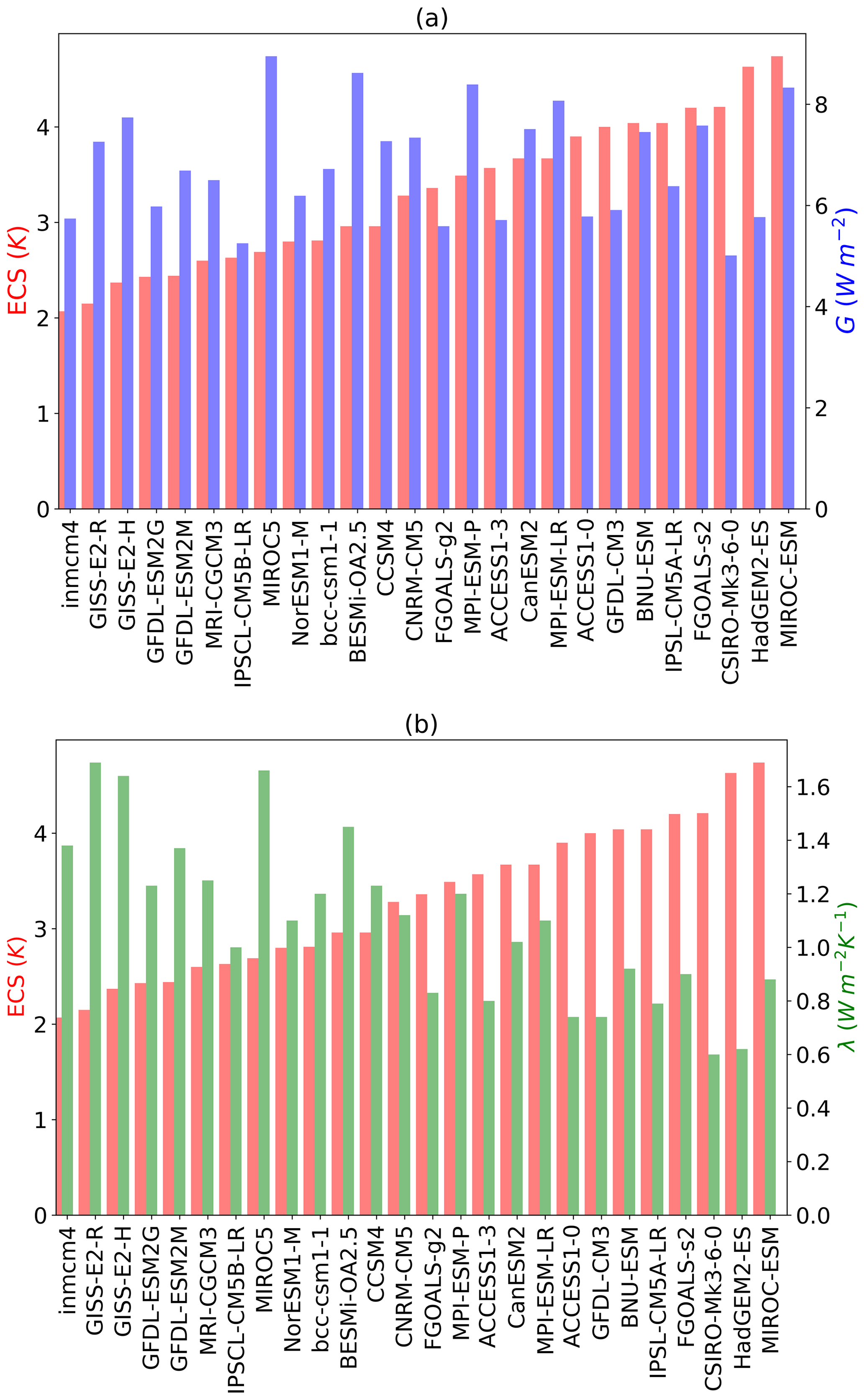
Figure 2(a) Equilibrium climate sensitivity (ECS, in red) and radiative forcing (G, in blue) values with ECS values increasing from left to right; (b) ECS (red) and climate sensitivity (λ, in green) with ECS values increasing from left to right.

Download

Table 3CO₂ forcing (W m⁻²) (G), net feedback (W m⁻² K⁻¹) (λ), climate response (W m⁻²) (ΔCRE), and equilibrium climate sensitivity (K) (ECS) values.

Download Print Version | Download XLSX

The ΔCRE from BESM is −0.13 W m⁻² K⁻¹, while the CMIP5 models yield ΔCRE values ranging from −0.50 to 0.70 W m⁻² K⁻¹. Unlike the ΔCRE_a, this term does not consider the masking effects of clouds as estimated via the radiative kernel method (Eq. 5). Therefore, the ΔCRE cannot be interpreted to reflect a change in the cloud properties alone.

4.2 Climate feedbacks estimated via the radiative kernel method

Figure 3 shows the global mean feedbacks for lapse rate, water vapor, lapse rate plus water vapor, albedo, and cloud (SW, LW, and total) for each CMIP5 model. Both radiative kernels are used to test whether the results are sensitive to the choice of radiative kernel and whether the inter-model deviation is greater than the distribution of the radiatively active constituents (temperature, water vapor, albedo, and cloud) of the base model. It is worth clarifying that positive (negative) values of feedbacks contribute to the amplification (damping) of global warming. The strongest positive feedback (Fig. 3) is due to water vapor (mean value: 1.39 W m⁻² K⁻¹), followed by clouds (mean value: 0.96 W m⁻² K⁻¹) and then surface albedo (mean value: 0.32 W m⁻² K⁻¹). The global mean Planck feedback is negative, with an average value of −3.60 W m⁻² K⁻¹ (not shown in Fig. 3), followed by a lapse rate feedback of −0.77 W m⁻² K⁻¹. BESM yields values near the ensemble mean for the albedo and cloud feedbacks, i.e., 0.27 and 0.95 W m⁻² K⁻¹, respectively. For the lapse rate feedback BESM yields a value of −0.71 W m⁻² K⁻¹, slightly underestimating the ensemble mean value in magnitude. In turn, BESM is among the models with the lowest global water vapor feedback average, with a value of around 1.24 W m⁻² K⁻¹.

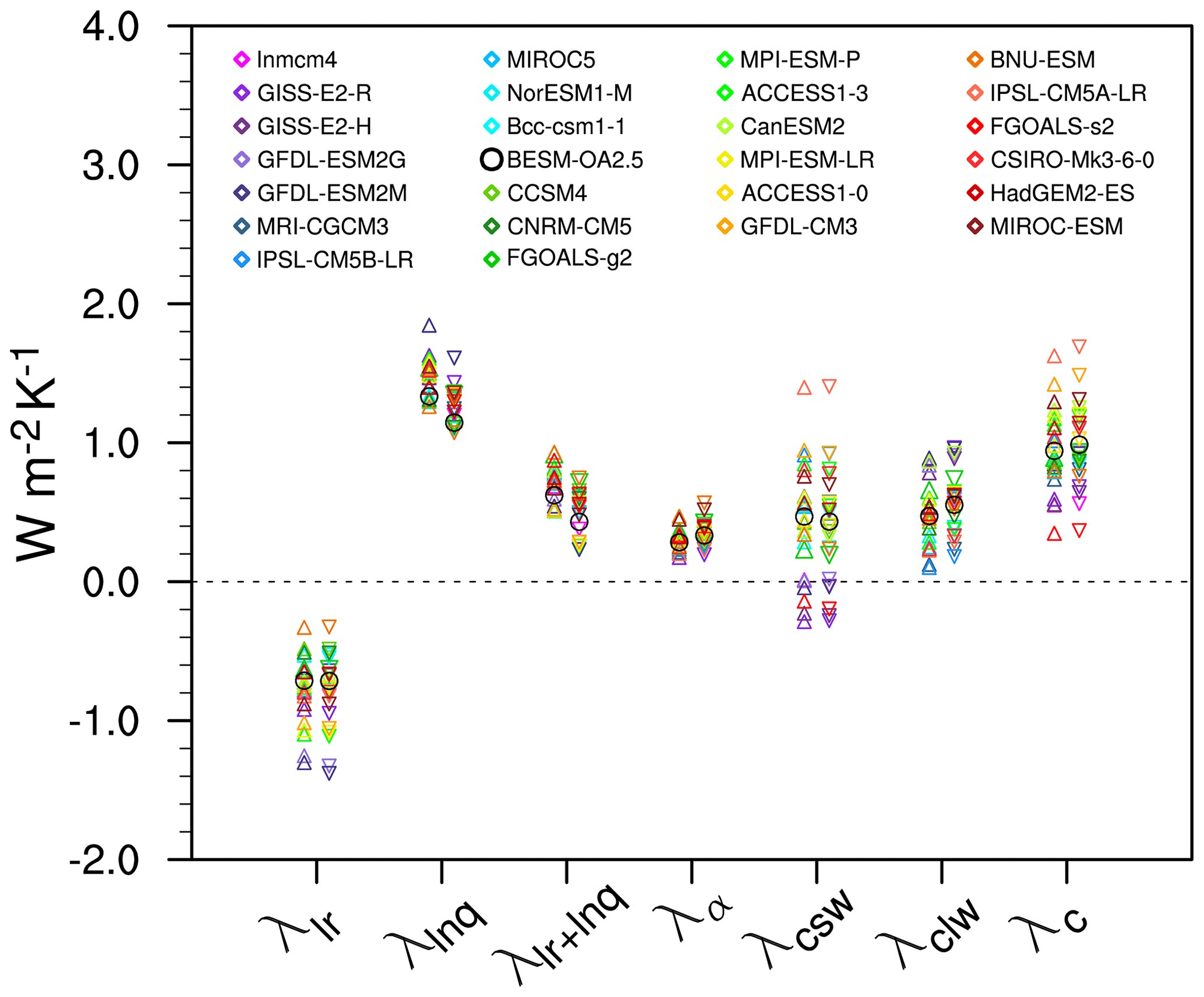
Figure 3Global mean feedbacks for 25 CMIP5 models and BESM-OA2.5 (circle). Changes in abrupt4xCO2 relative to the piControl were averaged over years 120–150. The triangles represent the mean estimated feedback values calculated using the NCAR radiative kernel, whereas the upside-down triangles represent the estimated feedback values calculated using the GFDL radiative kernel.

Download

Figure 4 shows the latitudinal profiles for the global mean feedback values in Fig. 3, allowing us to identify the regions that induce deviations of BESM results from the CMIP ensemble. In Fig. 4a–b, there is a nearly constant Planck feedback of approximately −3.4 W m⁻² K⁻¹ from 90 ^∘S to 60^∘N, with a notable increase in the ensemble standard deviation in the sub-Antarctic latitudes (around 60 ^∘S), which is in accordance with Rieger et al. (2017). The exception is in the Arctic region, where the mean value reaches −10 W m⁻² K⁻¹ with a similarly increased standard deviation value. In the sub-Antarctic and Arctic latitudes, BESM yields one of the most negative values for the Planck feedback, revealing that BESM has a stronger vertically homogeneous warming (corresponding to large surface warming) among the CMIP5 models. Furthermore, for those same regions, BESM showed more positive lapse rate feedback than the ensemble. Therefore, BESM yields a warming relatively larger at the surface and relatively weaker at the upper troposphere, resulting in a stronger vertical temperature gradient in comparison to the other models.

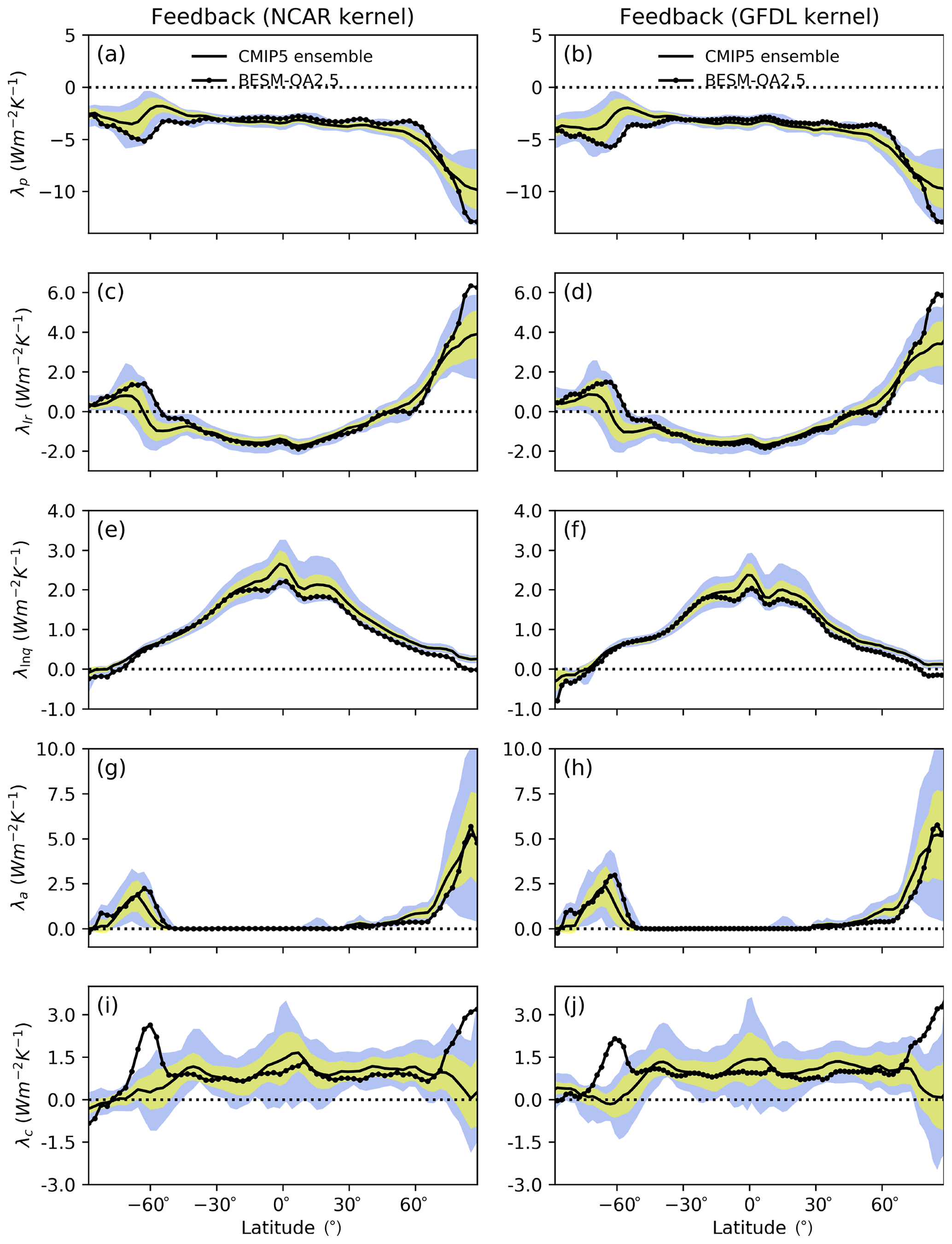
Figure 4Feedbacks for the CMIP5 multi-model ensemble mean (solid line) and BESM-OA2.5 (solid line with dots) for the Planck feedback (a, b), lapse rate feedback (c, d), water vapor feedback (e, f), albedo feedback (g, h), and cloud feedback (i, j). Inter-model standard deviations for each latitude are in yellow. In blue are the feedback limits based on the maximum and minimum values for each latitude among the models, excluding BESM-OA2.5. All feedbacks are based on the averaged over years 120–150.

Download

In the tropics, where there is an intense moist convection, atmospheric warming almost follows a moist adiabat (temperature increase is larger in the upper troposphere compared to that at the surface), implying a negative lapse rate feedback (Fig. 4c–d) (Manabe and Stouffer, 1980). In accordance with this upper tropospheric warming in the tropics, an increase in the specific humidity occurs (Manabe and Wetherald, 1975), which causes a reinforcement of the greenhouse effect, reflected by a positive water vapor feedback as shown in Fig. 4d–e. Because of this close link between the lapse rate and water vapor feedbacks, it is common to consider their effects as a sum, as displayed in Fig. 3. BESM shows a lapse rate feedback near the ensemble mean for the tropics. The greatest BESM deviations are observed near the Antarctic and over the Arctic (Fig. 4c–d), where this feedback became positive for all models. For the water vapor feedback, greater dispersion of the models was observed in the tropics, with BESM systematically yielding values below the ensemble mean for the same latitude band (Fig. 4e–f). These lower values extend throughout the Northern Hemisphere, consistent with the low global mean water vapor feedback value relative to the ensemble (shown in Fig. 3).

The albedo feedback profiles from BESM and the CMIP5 models are compared in Fig. 4g–h. Nonzero results mostly occur over the polar regions, where there is a reduction in sea ice and snow cover (Chung and Soden, 2015; Block et al., 2020). The positive albedo feedback signals yielded by all of the models in such regions imply that the reduction in the albedo corresponds to an increase in the radiation budget at the TOA due to reduced upward shortwave radiation. As expected, the polar regions present a large dispersion among the models, which is related to how fast the sea ice melts in the different climate models. The regions over the Arctic and the ocean near the Antarctic show the largest surface warming, and this positive albedo, together with the positive lapse rate feedbacks, is the main factor responsible for a phenomenon known as polar amplification (Pithan and Mauritsen, 2014; Block et al., 2020). BESM yielded an albedo feedback greater than the ensemble standard deviation over the Southern Ocean at around 60^∘ S. This same latitude is where BESM shows negative Planck and positive lapse rate feedbacks outside the models limits, as previously discussed.

Finally, regarding cloud feedback, most of the inter-model spread arises from the SW component (Figs. 3 and 4i–j). This dispersion is also reflected in the standard deviation and in the limit between the minimum and maximum of the zonally averaged cloud feedback shown in Fig. 4i–j. The SW cloud feedback ranges from −0.28 to 1.40 W m⁻² K⁻¹, while the LW cloud effect ranges from 0.10 to 0.96 W m⁻² K⁻¹. The combined SW and LW cloud effects result in positive cloud feedback ranging from 0.35 to 1.69 W m⁻² K⁻¹. This result is similar to that found by Soden et al. (2008) for CMIP3 (IPCC AR4, IPCC, 2007) models, who also reported a near-zero to positive cloud feedback. BESM presents positive values of around 0.5 W m⁻² K⁻¹ for both SW and LW cloud feedback, resulting in a total cloud feedback of about 1.0 W m⁻² K⁻¹ (as shown in Fig. 3). The highest positive values are in regions with strong albedo feedback (Fig. 4i–j).

Although BESM yielded global area-averaged feedbacks near the model ensemble mean values, differences are found mainly at high latitudes. In fact, for cloud feedback, BESM is an outlier due to a strong shortwave component response over both the Arctic and the Southern Ocean near the Antarctic. This effect is evident via the decomposition of the cloud feedback into the SW and LW components for the ensemble and BESM values, as shown in Fig. 5. To assess the analytical causes of this strong BESM shortwave cloud feedback departure from the ensemble, we separately computed the contributors to the SW cloud feedback, i.e., the SW CRE (as described by Cess et al., 1989) and the feedback cloud masks, as in Eq. (5). For the shortwave component, the feedback cloud masks are obtained for the albedo and SW water vapor feedbacks by calculating the all-sky minus clear-sky radiation flux for each feedback. We find that the higher BESM cloud feedback values (Fig. 6g–h) are mainly consequences of the sum of the SW CRE (Fig. 6a–b) and the effect of cloud masking for the albedo feedback (Fig. 6c–d) in the sub-Antarctic and Arctic regions. In turn, the cloud masking for the SW water vapor (Fig. 6e–f) does not contribute to the higher positive BESM values. As shown in Fig. 6, it is possible to attribute BESM's status as an outlier over the Arctic region to the SW CRE, while in the Southern Ocean (around 60^∘ S), the major contribution comes from the albedo feedback cloud mask.

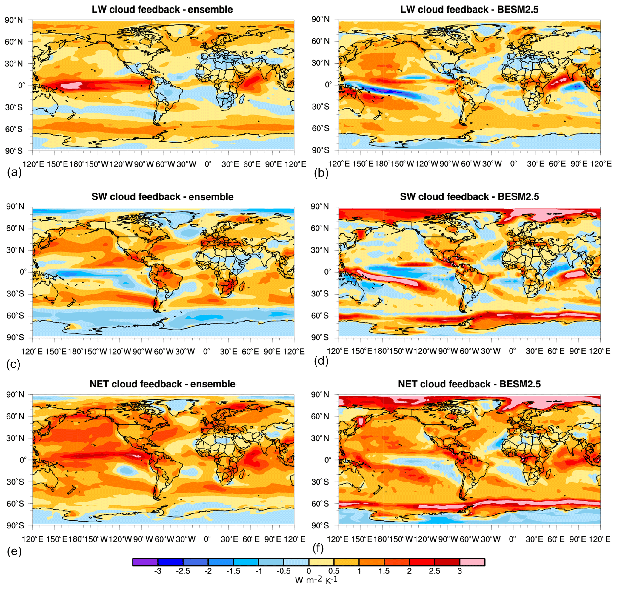
Figure 5Cloud feedbacks calculated using the NCAR radiative kernel for the CMIP5 ensemble (a, c, e) and BESM-OA2.5 (b, d, f). These results are based on the average from years 120–150.

Figure 6Shortwave cloud radiative effect (a, b), the albedo (c, d) and shortwave water vapor (e, f) feedback cloud maskings, and shortwave cloud feedback (g, h) for the CMIP5 multi-model ensemble mean (solid line) and BESM-OA2.5 (solid line with dots). Inter-model standard deviations for each latitude are in yellow. In blue are the feedback limits based on the maximum and minimum values for each latitude among the models, excluding BESM-OA2.5 (physical units of these feedbacks: W m⁻² K⁻¹).

Download

A deepened physical analysis to understand the BESM cloud feedback behavior in high latitudes is obtained by examining the zonal mean of the change in the cloud vertical profile for BESM, as shown in Fig. 7. Over the Arctic and near the Antarctic, BESM showed an increase in the cloud fraction above 850 hPa and a decrease below that level, indicating an upward shift of low-level clouds (Fig. 7a). However, the increase in cloud cover above 850 hPa is stronger than the reduction below. Because of this increase in the total cloud fraction, a negative SW CRE (not adjusted) appears in those regions (Fig. 6a–b), consistent with an increase in sun shading (Fig. 7b). Moreover, the SW cooling is smaller than the heating provided by LW radiation due to the upward shift of the low-level clouds, as evident in the net effect (Fig. 7d). Furthermore, the positive albedo and lapse rate feedbacks (Fig. 4c–f) are consistent with this vertical cloud shifting. In this manner, a loss of SW energy at the surface associated with an increase in the total cloud fraction explains the negative SW CRE, and the gain of LW energy is responsible for the sea ice melting. Consequently, this gain of LW energy is indirectly linked to the albedo feedback cloud mask for BESM, since the mask ($\mathrm{\Delta }a/\mathrm{\Delta }{\stackrel{\mathrm{‾}}{T}}_{\mathrm{as}}(K_a-K_a^{\mathrm{cs}})$) is proportional to the albedo change (Δa). As discussed before, both the SW CRE and albedo feedback cloud mask contribute to the large positive cloud feedback over the Arctic and sub-Antarctic areas observed in BESM.

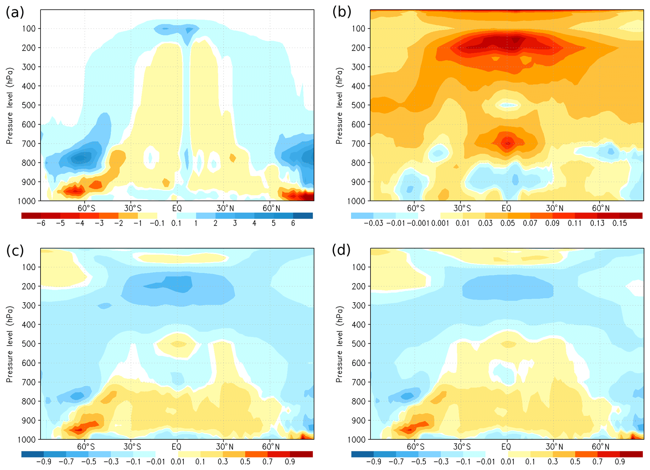
Figure 7Vertical profiles of the zonal mean of the abrupt4xCO2–piControl mean difference for the following variables: (a) cloud fraction; radiative heating or cooling rate (dT∕dt; K d⁻¹) of (b) shortwave, (c) longwave, and the (d) sum of the shortwave and longwave for BESM-OA2.5.

Download

4.3 Changes in temperature, atmospheric circulation, and precipitation

Figure 8 shows the annual mean surface temperature differences between the abrupt4xCO2 and piControl scenarios for the ensemble of 25 CMIP5 models and BESM. As clearly shown in Fig. 8, despite the generalized increase in the surface temperature over most of the globe, BESM shows a generally lower temperature increase, principally over the continental areas. The CMIP5 ensemble yields a mean continental temperature increase of 6.78 K, while BESM yields a value of 5.57 K. Nevertheless, the spatial patterns of the temperature increases are similar, as measured by the spatial inner product (as described in the previous section) between Fig. 8a and b, which results in a value of 0.96 (values near 1 indicate that both variables have a similar spatial pattern, whereas values near 0 mean that there is hardly any pattern correlation between variables). One point of interest within the scientific community is the relatively low temperature increase over the subpolar North Atlantic, also referred to as the warming hole (Drijfhout et al., 2012). In the CMIP5 ensemble mean, the North Atlantic does not show a temperature decrease, although it is the region with the smallest temperature increase globally, while BESM shows an area of temperature decrease in this region. Such a decrease is also present in six other analyzed models (CSIRO-Mk3-6-0, FGOALS-s2, GFDL-ESM2G, GFDL-ESM2M, GISS-E2-R, and inmcm4). These results are consistent with those of Drijfhout et al. (2012), who showed that both observations and CMIP5 models present maximum cooling in the center of the subpolar gyre. The authors argue that there is evidence that both the subpolar gyre and the AMOC adjust in concert with different time lags.

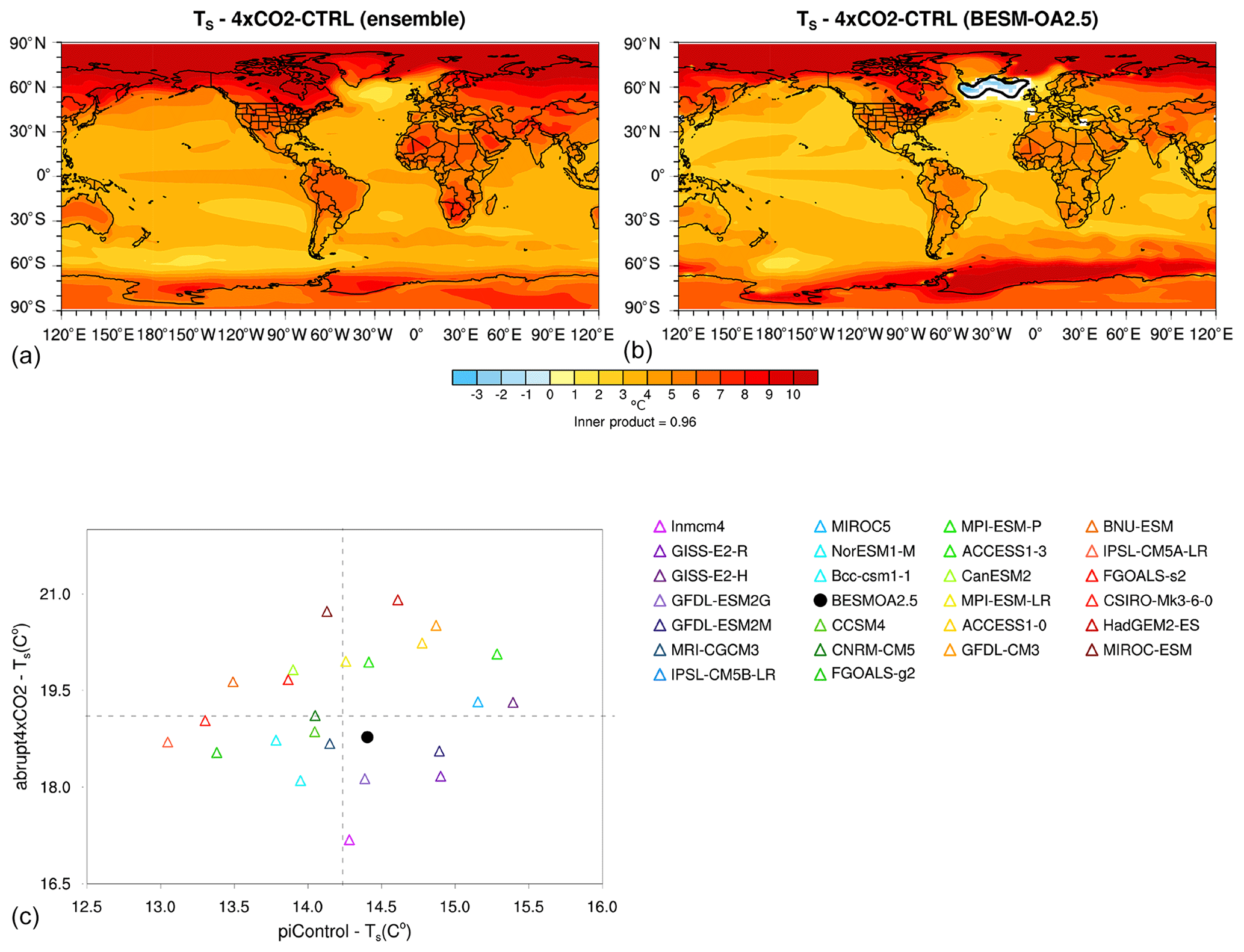
Figure 8Differences (averaged over years 120–150) in surface temperature between the abrupt4xCO2 and piControl simulations in (a) the CMIP5 ensemble and (b) BESM-OA2.5. (c) A scatter plot of the global average surface temperature for the CMIP5 models used in the ensemble and BESM-OA2.5 (black dot). The shaded areas in (a) and (b) have confidence levels greater than 90 %; the black line represents the contour line of zero temperature difference.

The regions with the largest temperature increase in the abrupt4xCO2 scenario are the polar regions, particularly over the Arctic. The equatorial Pacific shows a relative maximum in warming when the abrupt4xCO2 scenario is compared with the piControl both in the CMIP5 ensemble and BESM. Such changes in the Pacific mean state are consistent with the IPCC AR5, which reports that the Pacific Ocean becomes warmer near the Equator compared to the subtropics in the CMIP5 projections (Liu et al., 2005; Gastineau and Soden, 2009; Cai et al., 2015). The scatter plot of the global average under abrupt4xCO2 conditions versus the piControl conditions presented in Fig. 8 provides additional information that helps to understand the dispersion around the mean value among the different models. Even though the outputs of most of the models lie in either quadrant 1 or 3 (top right and bottom left, respectively), it is not possible to claim any robust linear relationship. This result indicates that models with warmer or cooler mean climates in the piControl runs apparently do not show a corresponding warmer or cooler climate in the abrupt4xCO2 experiments. BESM yields a temperature near that of the ensemble in both the piControl and abrupt4xCO2 runs; consequently, it also showed a temperature increase near the ensemble mean, consistent with its Planck feedback (Figs. 3 and 4a–b).

Figure 9 shows the precipitation changes between the abrupt4xCO2 and piControl scenarios for the multi-model ensemble and the BESM. The results are, in general, similar to those of Held and Soden (2006), with wet regions becoming wetter (near-equatorial and subpolar regions) and dry regions becoming drier (centered around 30^∘ in both hemispheres). The precipitation pattern in the CMIP5 ensemble shows increased precipitation over the equatorial Pacific, which could be related to the equatorial Pacific warming pattern shown in the temperature change (Fig. 8). Furthermore, the CMIP5 ensemble shows a decrease in precipitation in northern South America. The BESM precipitation pattern is similar to the spatial patterns in the CMIP5 ensemble but with some notable exceptions. For example, the decreased precipitation over the South Pacific shown in the CMIP5 ensemble plot is extended into the Indonesian region in BESM. It is also worth noting that in the BESM simulation, the South Pacific convergence zone (SPCZ) shifts southward in the abrupt4xCO2 scenario compared with its position in the piControl scenario. In both the multi-model ensemble and BESM, the precipitation change pattern over South America is similar to that which occurs during El Niño years (Kayano et al., 1988; Marengo and Hastenrath, 1993; Grimm and Tedeschi, 2009), with increased precipitation over southeastern South America and decreased precipitation over northern–northeastern South America. The scatter plot in Fig. 9 emphasizes a linear relationship between the experiments, indicating that models with higher (lower) global average precipitation in the piControl scenario show higher (lower) precipitation in the abrupt4xCO2 scenario. As is obvious from Fig. 9, the BESM performance perfectly matches the ensemble mean behavior in global mean.

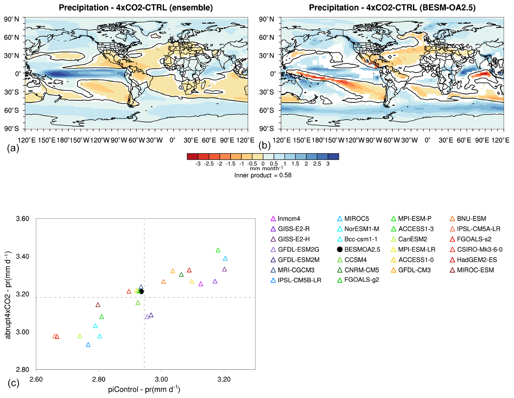
Figure 9Differences (averaged over years 120–150) in precipitation (mm month⁻¹) between the abrupt4xCO2 and piControl simulations in (a) the CMIP5 ensemble and (b) BESM-OA2.5. (c) A scatter plot of the precipitation global averages for the CMIP5 models used in the ensemble and BESM-OA2.5 (black dot). The shaded areas in (a) and (b) have confidence levels greater than 90 %; the black line represents the contour line of zero precipitation difference.

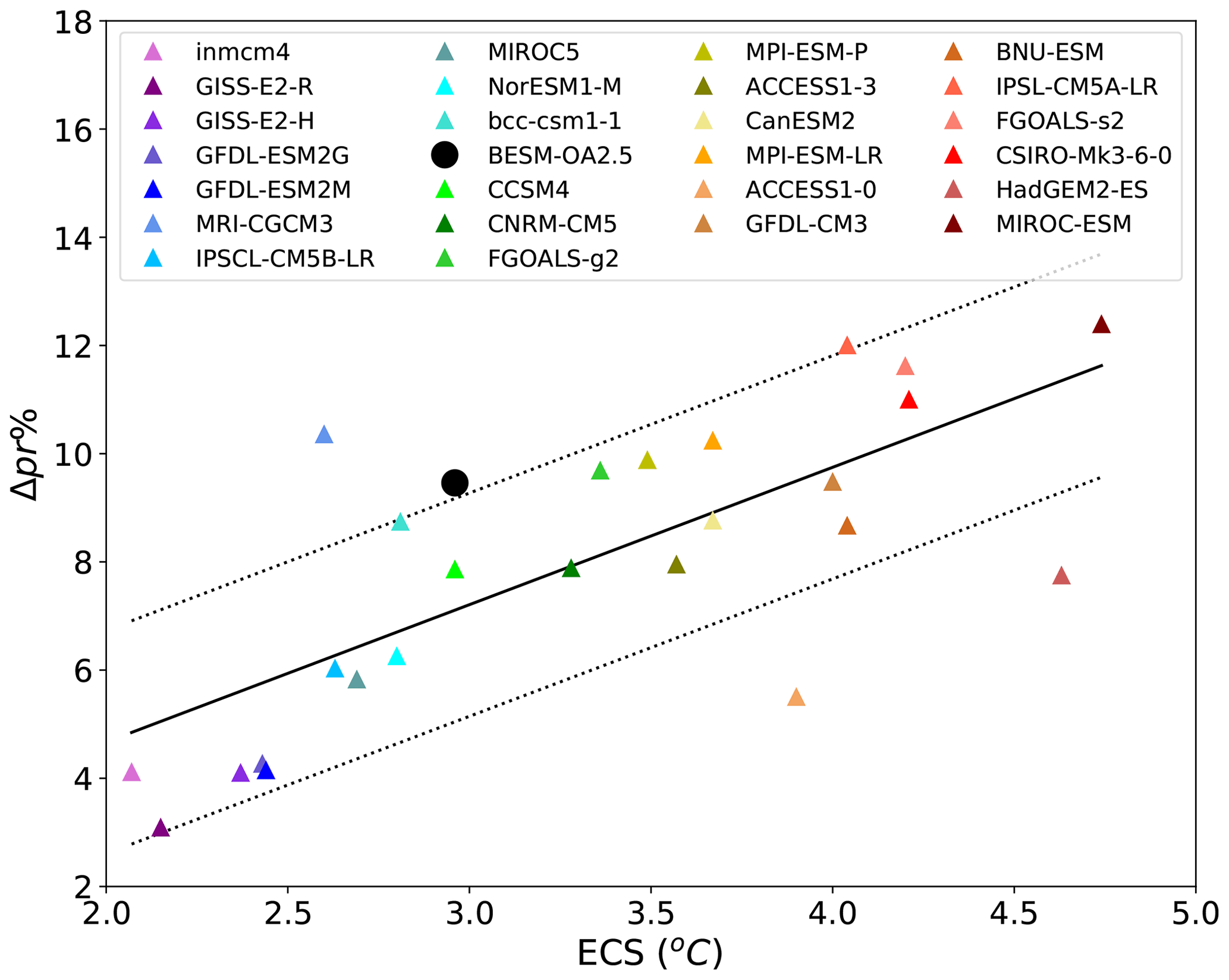
Figure 10Scatter plot of the ECS and ΔPr (%) values for all of the ensemble models. The solid black line shows the linear fit between the ECS and the perceptual precipitation change. As in Fig. 2, the models are sorted according their ECS value. The dashed lines represent the error limits considering the residual standard error.

Download

Figure 10 shows a scatter plot of the ECS versus the precipitation difference between the abrupt4xCO2 and piControl scenarios (ΔPr) for all of the considered models. It is worth noting that all the models show increased global mean precipitation upon a quadrupling of atmospheric CO₂ with piControl preindustrial CO₂ concentrations (positive values on the y axis in Fig. 10). An apparent linear relationship between these differences (abrupt4xCO2 minus piControl) in the global mean precipitation and ECS is also evident in Fig. 10, in which the warmest models tend to have the largest precipitation changes. The slope of the linear regression reflects a 2.5 % precipitation change per Kelvin, which is close to that found by Held and Soden (2006). This slope is much lower than that predicted by the Clausius–Clapeyron relation, i.e., an approximately 6.5 % change in precipitation per Kelvin. In fact, such precipitation increases are not governed by moisture availability but rather by the surface and tropospheric energy balance, which incorporates the surface radiative heating, surface latent heat flux, and radiative cooling of the troposphere (Allen and Ingram, 2002).

MRI-CGCM3, ACCESS1-0, and HadGEM2-ES show greater deviations from the linear fit shown in Fig. 10. Furthermore, BESM is marginally out of the residual standard error interval, with a 9.5 % increase in precipitation (the error limit is 9.2 %). ACCESS1-0 and HadGEM2-ES use the same atmospheric model (Bi et al., 2013; Dix et al., 2013), which could explain the lower increase in precipitation in both coupled models.

In addition to temperature and precipitation changes, we are also interested in understanding the changes in the BESM atmospheric circulation (compared to other models) following a quadrupling of the CO₂ concentration. The sea level pressure (SLP) response patterns shown in Fig. 11 depict a poleward shift in the subtropical high-pressure cells in both the CMIP5 ensemble and BESM. Furthermore, when the models are subjected to the increased atmospheric CO₂ concentration, a decrease in the SLP over the polar regions is evident. This, connected with the increase in the midlatitudes, indicates a positive trend in Arctic oscillation (AO) and Antarctic oscillation (AAO) episodes, which have already been reported by Fyfe et al. (1999), Cai et al. (2003), and Miller et al. (2006). It is also interesting to note the statistically significant SLP decrease (increase) over the eastern (western) Pacific, a pattern that might indicate an ENSO-like pattern in scenarios with an increased CO₂ concentration. This pattern is consistent with those depicted in Fig. 8 for the SST changes in a 4xCO₂ scenario.

Figure 11Difference (averaged over years 120–150) in sea level pressure (SLP; hPa) between the two scenarios (abrupt4xCO2 minus piControl; shaded) and SLP under piControl conditions (contours) in the CMIP5 model ensemble (a) and BESM-OA2.5 (b). The white areas have confidence levels less than 90 %.

The results from the piControl scenario (the contours in Fig. 12) show that the Southern Hemisphere subtropical jet, reflected by the core of the maximum eastward zonal wind, is localized around 35^∘ S at 200–150 hPa in both the CMIP5 ensemble and BESM. In Fig. 12a and b (BESM and the CMIP5 ensemble), we note that the regions with the strongest increases in westerly winds at all levels show a southward jet displacement. This observation is consistent with the poleward displacement of the high SLP center shown in Fig. 11. Furthermore, as the high-pressure centers experienced a poleward shift, the pressure gradients intensified in the subpolar areas; consequently, the near-surface wind velocity increased, following the geostrophic approximation ($u\approx -(\mathrm{1}/f\mathit{\rho })(\partial p/\partial y)$), where f is the Coriolis parameter and ρ is the air density.

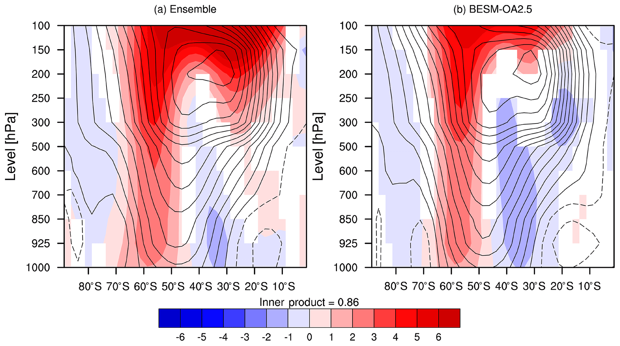
Figure 12Vertical profile of the difference (averaged over years 120–150) in the zonal wind (m s⁻¹) between the two scenarios (abrupt4xCO2 minus piControl; shaded) and the piControl conditions (contours) for (a) the ensemble of CMIP5 models and (b) BESM-OA2.5. The white areas have confidence levels less than 90 %.

Download

Figure 13 shows the average differences from 5^∘ N to 5^∘ S (Walker circulation) between the abrupt4xCO2 and piControl scenarios for vertical motion (omega; shaded) and zonal wind and vertical motion (vectors). According to the vertical motion pattern in the piControl (contours), the multi-model ensemble and BESM show subsidence over an extensive area in the Pacific (150^∘ E–90^∘ W) whose intensity is lower in the abrupt4xCO2 simulation, as shown in Fig. 13 (blue). This finding is coherent with near-surface temperature patterns (Fig. 8), which show an equatorial warming pattern in the mean state (e.g., during El Niño years, a weakening of the Walker circulation occurs). Furthermore, there is enhanced subsidence for the difference between the two scenarios over South America (around 75^∘ W), consistent with the decrease in precipitation in tropical South America, in both BESM and the CMIP5 ensemble (Fig. 9).

Figure 13Difference (averaged over years 120–150) between the abrupt4xCO2 and piControl conditions for generalized vertical motion (omega (Pa s⁻¹); shaded) and the mean zonal and vertical motion (vectors) averaged between 5^∘ S and 5^∘ N for (a) the CMIP5 ensemble and (b) BESM-OA2.5. The contours represents the averaged piControl vertical motion (omega) in the same region. The white regions have confidence levels less than 90 %.

Download