the Creative Commons Attribution 4.0 License.
the Creative Commons Attribution 4.0 License.
 | 26 May 2020
An online emission module for atmospheric chemistry transport models: implementation in COSMO-GHG v5.6a and COSMO-ART v5.1-3.1
Michael Jähn
Gerrit Kuhlmann
Qing Mu
Jean-Matthieu Haussaire
David Ochsner
Katherine Osterried
Valentin Clément
Emission inventories serve as crucial input for atmospheric chemistry transport models. To make them usable for a model simulation, they have to be pre-processed and, traditionally, provided as input files at discrete model time steps. In this paper, we present an “online” approach, which produces a minimal number of input data read-in at the beginning of a simulation and which handles essential processing steps online during the simulation. For this purpose, a stand-alone Python package “emiproc” was developed, which projects the inventory data to the model grid and generates temporal and vertical scaling profiles for individual emission categories. The package is also able to produce “offline” emission files if desired. Furthermore, we outline the concept of the online emission module (written in Fortran 90) and demonstrate its implementation in two different atmospheric transport models: COSMO-GHG and COSMO-ART. Simulation results from both modeling systems show the equivalence of the online and offline procedure. While the model run time is very similar for both approaches, input size and pre-processing time are greatly reduced when online emissions are utilized.
- Article
(4317 KB) -
Supplement
(498 KB) - BibTeX
- EndNote


Gridded and temporally varying emission fields are a critical input for three-dimensional atmospheric chemistry transport models (Matthias et al., 2018). Traditionally, such emissions are obtained from an inventory and pre-processed for the model as external inputs, which are read-in during simulation at regular time steps. The pre-processing typically includes a mapping of the inventory to the model grid and the application of temporal and vertical profiles depending on emission source category. In the case of atmospheric chemistry models, a speciation, i.e., a mapping of the species in the inventory to those simulated in the model, is required, for example the mapping of total non-methane volatile organic compounds (NMVOCs) to individual NMVOC species. A prominent example of an emission pre-processing model is the Sparse Matrix Operator Kernel Emissions model (SMOKE, https://www.cmascenter.org/smoke/, last access: 15 May 2020), which has been used extensively with different atmospheric chemistry models in the United States (McHenry et al., 2004; Wong et al., 2012), Europe (Borge et al., 2008; Bieser et al., 2011a), and Asia (Wang et al., 2011). More recent examples are the pre-processor PREP-CHEM-SRC (Freitas et al., 2011), the High-Elective Resolution Modelling Emission System (HERMES; Guevara et al., 2019), and the Harvard-NASA Emission Component v1.0 (HEMCO; Keller et al., 2014).
In the case of a large number of tracers and hourly input, the pre-processing and reading of the emission fields (hereafter referred to as “offline approach”) imposes a large computational burden in terms of input and output (I/O) operations and storage. An alternative is to apply the temporal and vertical profiles inside the model (“online approach”), which greatly reduces the number and size of input files and the corresponding I/O. This approach enhances the flexibility in setting up new model simulations since no new emission data need to be generated before the start of a simulation. Furthermore, meteorology-dependent emissions, such as emissions from residential heating depending on outdoor temperatures, can be incorporated more easily.
Here we present such an online emission module, which has been integrated into two different atmospheric transport models, both based on the regional numerical weather prediction and climate model COSMO (Consortium for Small-scale Modeling; Baldauf et al., 2011). The first model was developed for the passive transport of tracers such as long-lived greenhouse gases and is referred to as COSMO-GHG (Liu et al., 2017; Brunner et al., 2019). The second model is COSMO-ART (Aerosols and Reactive Trace gases; Vogel et al., 2009; Knote et al., 2011), which simulates the transport and chemistry of reactive gases and aerosols as well as two-way feedbacks between meteorology and chemistry. Both are fully integrated, online coupled models simulating the meteorology and the transport (and chemistry) of atmospheric constituents consistently in one single model (Baklanov et al., 2014). The module has also been incorporated into the model COSMO-ART-M7 (Glassmeier et al., 2017), which extends COSMO-ART with an optional simplified chemistry and aerosol scheme for climate applications, but this implementation will not be discussed here.
The purpose of this study is to present the conceptual framework of the online emission module, to demonstrate its suitability and flexibility for the simulation of greenhouse gases and air pollutants, and to show its equivalence to the traditional offline approach. Although the implementation of the module is specific to COSMO, the overall concept is generic and the code has been written in a modular way to facilitate integration into other (Fortran-based) model systems, for example as an extension to the recently developed emission module for ICON-ART (Weimer et al., 2017). The online module is composed of one Fortran module file, which interfaces with several routines of the standard COSMO model and its extensions GHG and ART as described later.
Furthermore, a separate Python package generates a small number of input files required for the simulation. Different from the offline approach, these files are read-in only once at the beginning of a simulation. The Python package also supports the generation of hourly input files for offline applications. This capability is used here to compare simulations with online and offline emission processing. In contrast to the Fortran module, the Python package is independent of the specific model implementation and, therefore, of potential use for other atmospheric transport model system. Models and inventories that are currently not covered by the Python package can be implemented in a straightforward manner.
The paper is organized as follows: Sect. 2 describes the functionality of the Python pre-processing package. Section 3 presents the implementation of the online emission module in the modeling systems COSMO-GHG and COSMO-ART and demonstrates its advantages based on three practical examples. Finally, Sect. 4 shows a performance assessment for both offline and online processing and demonstrates the equivalence of the two approaches based on two example simulations.
For the pre-processing of the input data required by COSMO, a separate Python-based tool named “emiproc” has been developed. The tool provides the mapping of gridded emission inventories to any desired COSMO grid (latitude–longitude grid with a rotated pole) or a regular latitude–longitude grid. Other projections could be implemented easily. It also generates the temporal and vertical profiles needed for the online computation of emissions. If desired, the tool is able to generate offline emissions, which may be useful for users if no online emission module is implemented in their model.
The overall workflow of the emission pre-processing is illustrated in Fig. 1 for both approaches. In the case of offline emissions, an additional step is required for the interpolation to the vertical grid of COSMO, which is executed by the official COSMO pre-processing tool int2lm (http://www.cosmo-model.org/content/model/documentation/core/int2lm_2.05.pdf, last access: 15 May 2020). Int2lm also merges the emission fields with other COSMO inputs such as initial and boundary conditions and ensures proper formatting of the files.
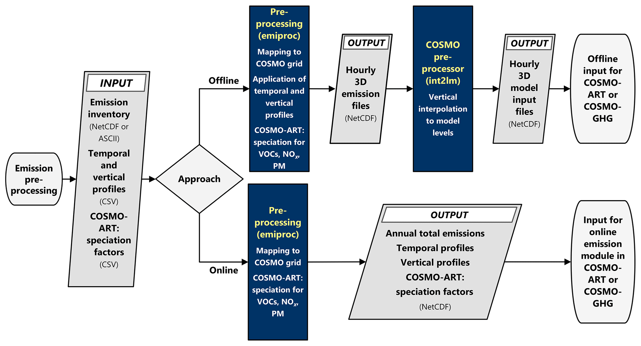
Figure 1Flow chart of the emission pre-processing for both offline and online approaches as implemented in COSMO-GHG and COMSO-ART. Dark gray parallelograms represent data (with input or output indicated). Blue rectangles are processing scripts. Start and end points are represented by ovals.
2.1 Gridded emission inventories
Emission inventories of greenhouse gases and air pollutants are usually provided as annual 2D gridded fields per source category (e.g., traffic, industry, residential, agriculture) (Kuenen et al., 2014; Janssens-Maenhout et al., 2017; Crippa et al., 2018). Before incorporating these emissions into a 3D atmospheric transport model, the 2D fields have to be convolved with temporal profiles of diurnal, day-of-week, and seasonal variability as well as with vertical emission profiles (Denier van der Gon et al., 2011; Pouliot et al., 2012; Kuenen et al., 2014). Current approaches for the definition of temporal and vertical profiles are often highly simplified (Matthias et al., 2018), partly due to a lack of detailed information but also due to the limited flexibility offered by the offline approach. Our current implementation of the module supports three different families of emission inventories: the inventories of the Netherlands Organization for Applied Scientific Research (TNO), the EDGAR inventories of the European Joint Research Centre (JRC), and the Swiss national emission inventories generated by Meteotest Inc., Switzerland. An extension to similar gridded inventories should be straightforward.
Although the inventories share a similar logic, there are distinct differences that had to be accounted for: in Europe, the two most prominent source classifications are the Standardized Nomenclature for Air Pollutants (SNAP; Centre on Emission Inventories and Projections, 2018) and the gridded Nomenclature for Reporting (GNFR; United Nations Economic Commission for Europe, 2015; Schindlbacher et al., 2016). SNAP is an old standard introduced in the context of the Convention on Long-Range Transboundary Air Pollution (CLRTAP), which had been used for many years in inventories produced by the European Monitoring and Evaluation Programme (EMEP) and by TNO. The latest inventories, however, follow the EMEP/CORINAIR NFR, which was introduced to harmonize the source classification with the one used in National Inventory Reports to the United Nations Framework Convention for Climate Change (UNFCCC EEA, 2000). For gridded inventories, the large number of NFR categories are usually lumped into 13 individual classes (A–M). This reduced set of categories is commonly referred to as gridded NFR or GNFR. EDGAR inventories are reported as individual or lumped NFR categories, which are similar but not identical to the GNFR standard. A table for unambiguous mapping between individual NFR, GNFR and SNAP categories is available at the United Nations Economic Commission for Europe (2003).
Another difference is the map projection. EDGAR and TNO inventories are reported on a regular latitude–longitude grid and the Swiss Meteotest inventories on a Cartesian grid in the Swiss CH1903 oblique Mercator projection. Furthermore, TNO inventories differentiate between point and area sources, which is not done in the other inventories. Point sources as reported to the European Pollutant Release and Transfer Register E-PRTR (https://prtr.eea.europa.eu, last access: 15 May 2020) are provided in the TNO inventories at their exact location, which has the advantage that in high-resolution simulations the point sources can be assigned accurately to the respective model grid cell. In addition, this allows applying separate vertical profiles to point and area sources as shown in Sect. 3.3.2.
2.2 Mapping to COSMO grid
All emission data need to be mapped onto the simulation grid, which in the case of COSMO is a rotated latitude–longitude grid. Such mapping is straightforward for point sources for which the emissions are added to the COSMO grid cells that contain the sources. For area sources this is less trivial, since simple interpolation is not mass-conservative, whereas conservative nearest-neighbor methods may lead to undesired stripes or other discontinuities. In order to avoid such issues and to accurately conserve mass, we determine the relative fraction of the overlap with each inventory grid cell for each COSMO grid cell. The emissions for all source categories s at each COSMO grid cell i are then computed by
where and are the emissions (in mass∕cell) at the ith and jth COSMO and inventory grid cell, respectively, N is the number of grid cells in the inventory, and fi,j is the dimensionless fraction of the source cell j contributing to destination cell i. The fraction is determined by computing the area of the intersection between each COSMO and inventory grid cell divided by the total area of the inventory cell using the equal-area Mollweide projection to conserve mass.
Our tool does not redistribute the low-resolution inventory data onto the high-resolution COSMO grid using additional information, such as land–sea masks and country boundaries, which can be used for improving the spatial allocation of area sources. This feature could be implemented in a future version similar to the implementation in the CHIMERE-2017 model (Mailler et al., 2017).
The generated netCDF file contains 2D gridded fields Ei,s directly on the COSMO grid. This file also contains a corresponding 2D country mask, which is an integer field with each grid cell being assigned the number of the country that has the largest fractional area. The unit of the emissions depends on the actual model and is converted accordingly. For example, COSMO-GHG expects kilograms per square meter per second, whereas emissions in COSMO-ART are in kilograms per hour per cell.
2.3 Temporal and vertical profiles
The emission of a tracer X at time t is calculated as the sum over the emissions per source category scaled with source-specific temporal scaling factors. A tracer is defined here as a quantity that is transported in the model, which can be a single trace gas or aerosol component, a composition of several species, or an idealized tracer. The temporal scaling factor for tracer X, source category s, and time t is generally given by
where , , and are diurnal, day-of-week, and seasonal scaling factors, respectively. The three scaling functions are dimensionless and have a mean value of 1, such that the mean value of all scaling factors applied to a full year of data is 1 (or very close to 1). The step functions h(t), d(t), and m(t) are the hour of the day, the day of the week, and the month of the year corresponding to the continuous time t, respectively. The emission of X at time t is thus
where EX,s is the annual mean emission flux of X of source category s (which is the basic field usually provided by an inventory) and n is the total number of source categories. This formula is applicable to an emission from a single grid cell or to a complete 2D emission field; i.e., EX and EX,s may be 2D fields. The functions may further depend on the country of the source. In that case, a further summation over countries is needed in combination with country masks. Our Python package and online emission module support country-specific time functions.
The generated netCDF files contain time functions of diurnal, day-of-week, and seasonal variations per tracer and source category. These scalings are provided in three separate files by default. However, it is also possible to provide only one file with hour-of-year scaling factors. The temporal profile variables are arrays with the two dimensions time (e.g., 24 different hourofday in the case of a diurnal profile) and country. If no country-specific information is available or desired, a uniform country mask with a single value for the whole model domain needs to be generated. Vertical profiles, in contrast, are 1D arrays with level as the only dimension, since they are not expected to vary with country.
With this approach, real trace gases such as CO2 can be simulated but so can idealized tracers representing only a subset of sources, for example a tracer representing only traffic CO2 emissions, by only summing over a subset of source categories in Eq. (3).
Emissions do not only occur at the surface but should be treated in 3D (Bieser et al., 2011b; Brunner et al., 2019). This is particularly true for elevated emissions from power plants or air traffic. Idealized vertical scaling functions vs are available for anthropogenic emissions, which distribute the emissions from a source of category s over a discrete set of geometric vertical layers (altitude relative to ground). The scaling factors add up to 1 when summed over all vertical layers. Examples are given in the Supplement. The emission of the simulated tracer X at time t and in vertical layer k is then given as
The file generated by the Python tool contains vertical profiles per tracer and source category. The number of levels and their heights above surface can be set independently of the vertical structure of the COSMO grid. The vertical profiles do not depend on time t in the current implementation of the module. This could be implemented in the future, for example to account for a meteorology-dependent plume rise of emissions from power plants.
2.4 Speciation
The chemical compounds simulated in COSMO-ART include species for which inventories provide direct emission strengths (e.g., SO2 or NH3). However, for other species, the inventories only provide aggregated information for a family of compounds. This is the case for NOx (sum of NO and NO2), NMVOCs, and particulate matter with a diameter of less than 2.5 µm (PM2.5) and 10 µm (PM10) (sum of various organic and inorganic aerosol compounds).
Therefore, to compute the emission of an individual compound simulated in the model, chemical speciation factors have to be applied to the total mass of the family. These speciation factors are specific for different source categories, since, for example, the composition of NMVOCs, PM, and NOx emissions is different for traffic and residential heating. Furthermore, the speciation factors depend on the specific chemical mechanism applied in the model, which determines the mapping between real and model-simulated species. Starting from Eq. (4), considering a simulated tracer X whose emissions are reported under a chemical compound with a speciation factor (dimensionless), the emission of X at vertical level k is given by
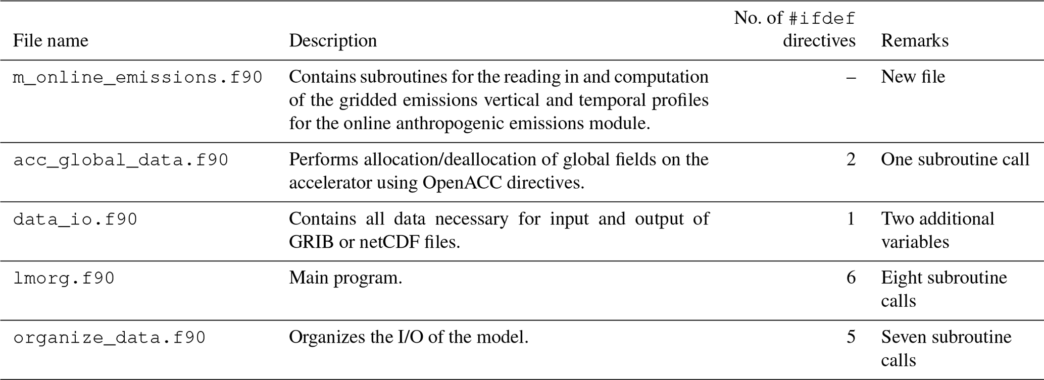
The online module was implemented in two extended versions of COSMO: COSMO-GHG developed for the simulation of passive tracers (e.g., greenhouse gases) and COSMO-ART for reactive trace gases and aerosols. An early version of the COSMO-GHG extension was developed in the CarboCount-CH project (Liu et al., 2017). It was built atop a generic tracer module, which was introduced in COSMO version 5.0 to enable a flexible definition of tracers with specific properties defined by their metadata (Roches and Fuhrer, 2012). In the standard weather prediction version of COSMO it is used for the advective, convective, and turbulent transport of all moisture tracers (water in the gas phase and in different hydrometeor phases). However, the life cycle of a tracer usually also involves other aspects not considered in COSMO, such as emissions or removal from the atmosphere. In the GHG extension, emissions can be supplied in the form of 2D surface fluxes or 3D volume emissions. To activate the GHG extension, COSMO has to be compiled with the -DGHG flag to enable the #ifdef GHG directives. Table 1 summarizes those interfaces to the GHG extension, including subroutine calls and number of #ifdef directives in the COSMO code.
Recently, the standard, CPU-based (central processing unit) COSMO version released by the German Weather Service has been fully ported to GPUs (graphics processing unit) (Fuhrer et al., 2014). This efficient GPU-enabled code, called COSMO-POMPA (Performance On Massively Parallel Architectures), is used operationally by the Swiss Federal Office of Meteorology and Climatology (MeteoSwiss) for daily weather forecasting. COSMO-POMPA has been integrated into the official version of COSMO since its release 5.5b, which can be compiled for both CPU- and GPU-based systems.
In order to benefit from the high efficiency of the GPU-enabled code, the GHG extension was ported to GPUs in the framework of the project SMARTCARB (Brunner et al., 2019). The porting was done using OpenACC compiler directives, which is a high-level approach to offload compute-intensive parts to a GPU accelerator (Lapillonne and Fuhrer, 2014). The same approach was employed for the porting of the online emission module. COSMO-GHG is available for COSMO version 5.6a, and it is planned to be integrated continuously for all upcoming releases of COSMO. Since COSMO 5.6a can be compiled for both CPU- and GPU-based platforms, the GHG extension and the online emission module had to be programmed in a way that they can be executed on both platforms as well. Depending on the chosen platform, code sections related to OpenACC directives are included or excluded from compilation based on #ifdef _OPENACC compiler directives.
COSMO-ART was developed at the Karlsruhe Institute of Technology for the simulation of air pollutants and their interactions with meteorology (Vogel et al., 2009; Knote et al., 2011). The ART extension makes use of the same generic tracer mechanism implemented in COSMO but adds an additional layer (a structure art_species) allowing for a more comprehensive definition of tracer properties such as molecular weight, initial and boundary values, and deposition properties. For each ART species, a corresponding tracer is generated and dynamically allocated in memory. The position of the associated tracer is referenced by an index in the art_species structure. Because the ART extension has not yet been ported to GPUs, COSMO-ART does not run with COSMO 5.6a but with the older release 5.1.
3.1 Basic framework for online emission processing in COSMO
The main philosophy is to read in all input data required for the online emission module only once at the start of the simulation. These data include annual mean sector-specific 2D emission fields EX,s as well as the temporal, vertical, and speciation profiles. During the simulation, these profiles are applied online to update the hourly emissions for each species according to Eqs. (2)–(5).
Table 2Members of the GHGCTL and OAECTL namelist group required in INPUT_GHG for COSMO-GHG and INPUT_OAE for COSMO-ART, respectively, for setting up the online emission module.
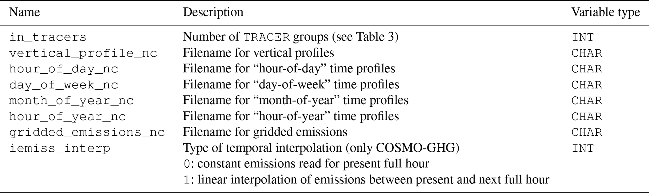
Table 3Namelist members of the TRACER group in INPUT_GHG and INPUT_OAE. Some namelist members are only implemented in COSMO-GHG or COSMO-ART.
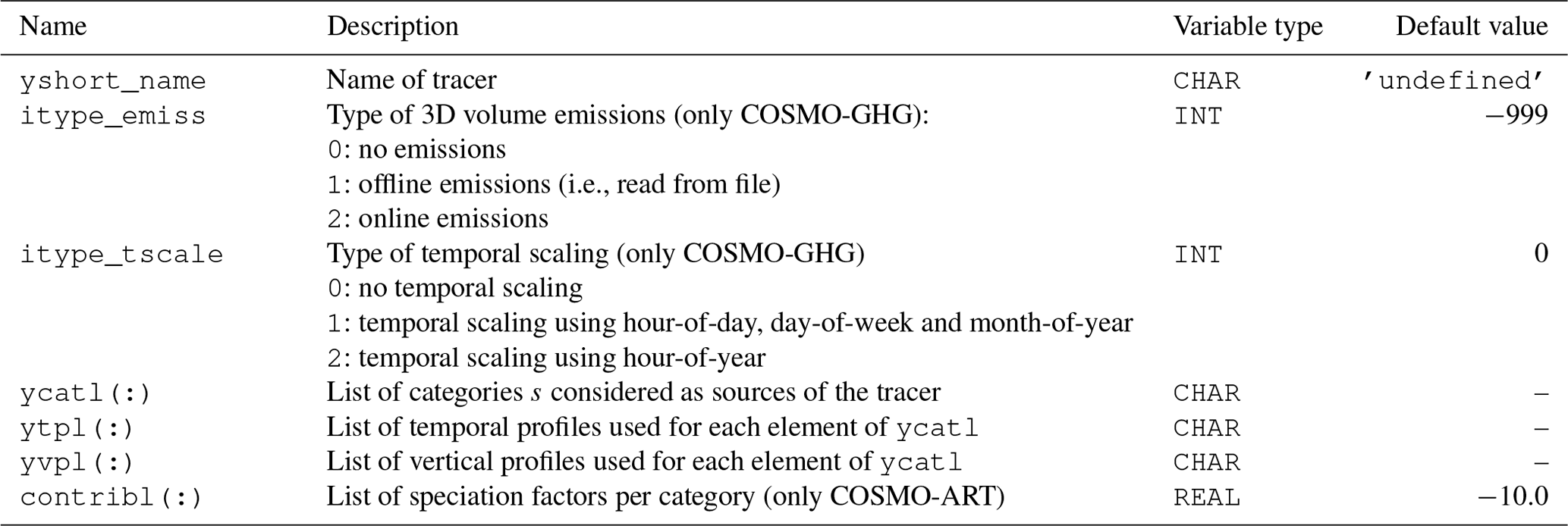
In order to implement new tracers flexibly, TRACER groups were added to the INPUT_GHG namelist file. A subset of the possible entries (members) of the TRACER group is presented in Table 3 and an example namelist file is given in the Supplement. For the online emission module, the definition of the TRACER group was extended with the following parameters:
-
a new possible value for the switch
itype_emiss, which needs to be set to2to activate online emissions for this tracer -
a list tag
ycatllisting the categories s considered as sources of the tracer -
a list tag
ytpllisting the temporal profile used for each element ofycatl -
a list tag
yvpllisting the vertical profile used for each element ofycatl -
a list tag
contriblused for chemical speciation, which lists the contribution of categories s to the total emitted mass of the tracer (only COSMO-ART).
Note that the comma-separated lists ycatl, ytpl, yvpl, and contribl need to have the same length. In contrast to COSMO-GHG, the definition of tracers is fixed (i.e., hard-coded) in COSMO-ART, and, therefore, no namelist file INPUT_GHG exists. In order to enable the same functionality as in COSMO-GHG, a new namelist file INPUT_OAE was introduced, where for each emitted tracer a corresponding TRACER group has to be defined (OAE: online anthropogenic emissions). In order to enable or disable the use of online emissions in COSMO-ART, a new Boolean switch lemiss_online was implemented in the namelist file INPUT_ART, which needs to be set to .TRUE. to activate the online emission module. For this reason, the namelist switch itype_emiss does not exist in COSMO-ART. The same applies for itype_tscale, since temporal scaling is applied just for hour-of-day, day-of-week, and month-of-year profiles.
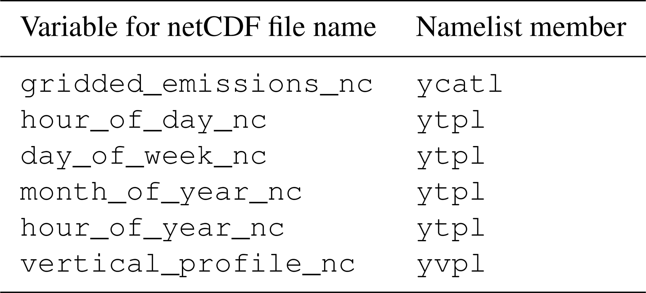
At the start of a simulation, the online emission module reads in the emission fields and the temporal and vertical profiles from the netCDF files generated by the Python tool, which have been described in Sect. 2. Full paths of the files have to be specified in the namelist file INPUT_GHG or INPUT_OAE; see Table 2. Note that variable names within the netCDF files have to be identical with those listed in ycatl, ytpl and yvpl, as shown in Table 4.
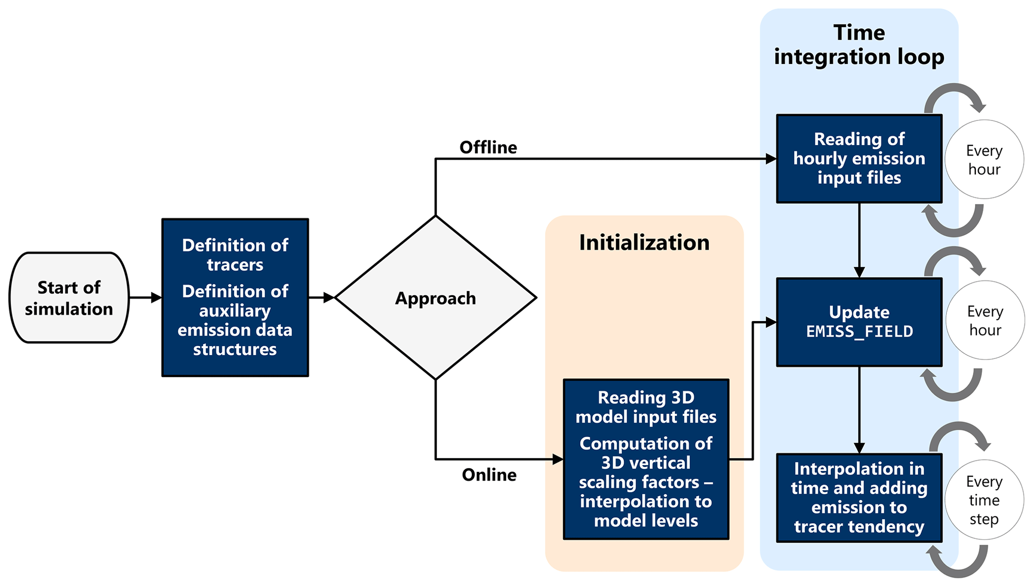
Figure 2Flow chart for COSMO-GHG run-time processes both for the offline and the online approach. Blue rectangles are code parts. The simulation start point is represented by an oval.
Table 4Overview of netCDF files and corresponding namelist tags in the TRACER group in INPUT_GHG or INPUT_OAE. The netCDF variable names must be identical to those listed in the namelist members (right column).
Speciation profiles for COSMO-ART are not provided in a separate netCDF file but are included in the namelist file INPUT_OAE through the list tag contribl of the TRACER group.
3.2 Modifications to the COSMO-GHG and COSMO-ART codes
In order to enable the computation of online emissions as an alternative to the default offline reading of emission files, the greenhouse gas module of COSMO-GHG (m_online_emissions.f90) was extended with new structures to store the information on temporal and vertical profiles and the annual mean sectorial emission grids. The arrays for temporal profiles and the emission grids are dynamically allocated as they depend on the tracer type. The information from the netCDF files is read at the beginning of the simulation. The vertical scaling factors, which are defined for layers above ground of fixed vertical extent (see Supplement), need to be translated into scaling factors for the vertical layers of COSMO. Since COSMO uses a spatially fixed grid with geometric hybrid vertical layers with thicknesses varying with the underlying topography, the vertical scaling factors are translated into dynamically allocated 3D arrays.
Before the implementation of the online emission module in COSMO-GHG, emissions were read-in every hour from a file and assigned to an emission field associated with each tracer. In COSMO-GHG, fields that are conceptually attached to a prognostic variable of the model (e.g., an emission field attached to a tracer) are called associated fields. The definition, memory management, and I/O aspects of associated fields are handled in src_associated_fields.f90. There, besides the already existing functionality of reading in files, a mechanism was added to compute the emissions based on the dynamically allocated arrays for the emission grid and temporal and vertical scaling factors. Afterwards, no matter if online or offline emissions are used, the emission fields are updated at the beginning of each hourly interval. The updates account for the new temporal scaling for the current hour and the 3D vertical scaling factors calculated at the beginning of the simulation by applying Eq. (4). The emissions are then kept constant during the current hour or linearly interpolated in time between the current and the next hour (if iemiss_interp is set to 1). The latter requires the computation (or reading) of the emission field at the following full hour. Finally, the emission field is added to the tracer tendencies at each model time step. All relevant computations in the GHG module use OpenACC directives in a similar manner as in other parts of the main COSMO code.
A schematic of all relevant processes for offline and online emissions in COSMO-GHG during model run time is shown in Fig. 2.
Even though the concepts are very similar, the realization of the online emission module in COSMO-ART differed significantly from the implementation in COSMO-GHG. The emission module in ART (art_emiss_prescribed.f90) comes on top of the tracer module in COSMO and interacts closely with the tracer fields in other ART modules such as art_mademod.f90 for aerosol processes. It was therefore desirable to keep most of the functionality of the standard emission modules to ensure the usability of both online and offline emission versions. The online emission module in COSMO-ART works as follows, focusing on the differences to the COSMO-GHG implementation: During initialization of the model, if the namelist parameter lemiss_online is set to .TRUE., the required files (emissions, temporal and vertical scaling factors) are read-in as described in Sect. 3.1. For every tracer with online emissions, the gridded emissions, the scaling factors (temporal and vertical), speciation values are collected in a data structure that associates this information with the location of that tracer in the art_species structure. Then, at hourly intervals during the run, the emissions are calculated and written into the corresponding array in art_species. Because this replaces the
assignment of emissions read-in from external files to the same array as done in the standard offline version, no further changes to other modules are required. It is even possible to mix on- and offline emissions in a simulation run, such that emissions of certain tracers are read-in, while others are calculated.
3.3 Practical examples
3.3.1 Merging of inventories
For regional-scale simulations it is often desired to merge different inventories covering different regions, e.g., nesting the high-resolution Swiss national inventory into the coarser European inventory of TNO. Two different approaches have been implemented in the Python tool to tackle this use case. For both approaches, the different inventories have to be mapped individually to the model grid using the Python tool as a first step. Afterwards, the inventories may be merged using a country mask by overwriting the data of the coarser inventory with the data from the high-resolution one for all grid cells corresponding to the selected country (or region). A simpler approach is to make use of the fact that temporal profiles can be country-specific. To merge the two inventories during the online processing, the hourofday profile for the coarse inventory can be set to 0 for the country covered by the high-resolution inventory and vice versa.
3.3.2 Distinction between area and point source emissions
The inventories of TNO differentiate between area and point source emissions. Point source emissions as reported to the European Pollutant Release and Transfer Registry (E-PRTR) correspond to strong local sources, which are often emitted from tall stacks. An example is emissions from residential heating, which can originate from large centralized facilities (possibly reported to E-PRTR) or from individual houses (reported as area sources). It may be desirable to apply different temporal and vertical profiles to these different types of sources. The Python tool allows generating separate grid maps and temporal and vertical profiles for point and area sources. Using these different maps and profiles for a given tracer is then straightforward, since point and area sources can be treated like separate source categories that need to be listed in the ycatl, ytpl, and yvpl tags of the tracer namelist group.
3.3.3 Modification of temporal and chemical speciation profiles
In a study of Athanasopoulou et al. (2017), the effect of the financial crisis in Greece on domestic fuel use and air pollution was investigated as an air quality modeling study using COSMO-ART. Due to the financial crisis, there was a sharp increase in wood burning for residential heating, which had major implications for air quality in Athens. Based on measurements of black carbon in the city, it became clear that the standard temporal profiles had to be updated to better reflect the actual burning of wood. For example, the standard profiles for residential heating predicted peaks of similar amplitude in the morning and evening and a minimum during weekends. This largely contrasted with the measurements which suggested maximum usage during weekends and a major peak in the evening but not in the morning. Furthermore, the speciation of PM2.5 emissions had to be modified, since wood burning emissions contain a large proportion (approx. 80 %) of primary organic aerosols. Adjusting the temporal and speciation profiles required changes to the emission pre-processing software and regenerating all hourly input files for the simulation. Using the online emission module, the same could have been achieved by a simple replacement of the temporal profiles in the netCDF files and of the speciation profiles in the namelist file INPUT_OAE.
Two sets of simulations comparing the results of online and offline emission handling using COSMO-GHG and COSMO-ART, respectively, are presented in the following. The comparison is made in terms of performance (computation time and storage requirements) and in terms of simulated tracer fields. Ideally, the two approaches should lead to identical results, but as will be shown, small numerical errors, e.g., due to the truncation of floating point numbers were found to produce small differences.
4.1 COSMO-GHG
Using the COSMO-GHG model with online and offline setup, respectively, a simulation with a single CO2 tracer for a domain covering the Alpine region at (≈1.1 km) horizontal resolution and with 60 vertical levels was conducted. The simulation extended over a period of 1 week from 1 to 8 January 2019. The boundary conditions for meteorological fields were taken from COSMO-7 reanalyses provided by MeteoSwiss. The CO2 tracer field was initialized to 0.
The model setup closely followed the settings of the operational high-resolution COSMO-1 forecast of MeteoSwiss. The simulations were performed on 60 hybrid CPU–GPU nodes of the Piz Daint supercomputer of the Swiss National Supercomputing Centre (CSCS). Each node included an Intel Xeon E5-2690 v3 12-core CPU and an NVIDIA Tesla P100 GPU.
The yearly gridded anthropogenic emissions of CO2 were taken from the TNO-GHGco (Super et al., 2020) inventory for 2015 available at resolution. They were split into 12 GNFR categories. The F category for road transport was further divided in three subcategories depending on the type of vehicles. Over Switzerland, the TNO inventory was replaced by a Swiss CO2 inventory at 500 m×500 m resolution, which was created by the company MeteoTest in the framework of the CarboCount-CH project (Liu et al., 2017). Due to a different source categorization used in the Swiss inventory, those categories were mapped to the GNFR categories B, C, F, J, and L. The temporal profiles applied to the emissions are described in the Supplement. No vertical profiles were applied in this example, but all emission were released at the surface. The namelist definition of the tracer in this simulation is described in the Supplement.
An example of the distribution of the simulated CO2 tracer representing all anthropogenic emissions in the domain and of the differences between online and offline is shown in Fig. 3. The figure shows instantaneous near-surface CO2 at the end of the 7 d simulation period.
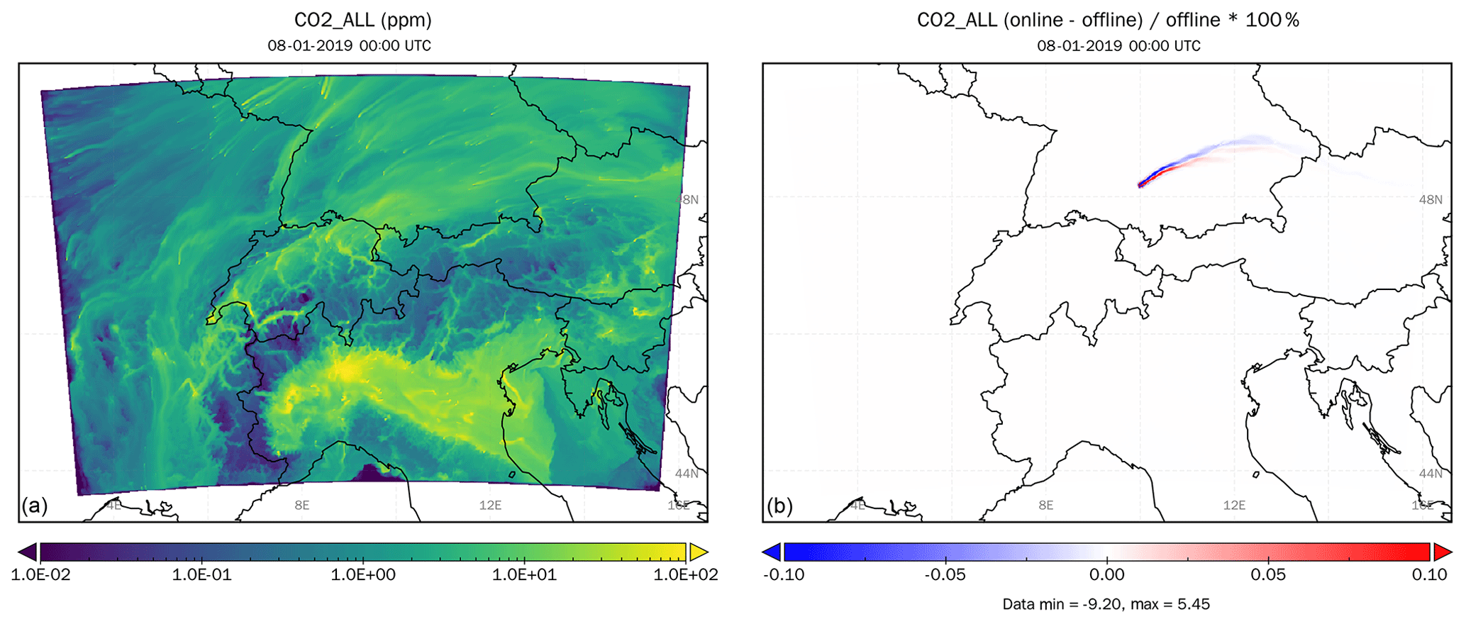
Figure 3Surface-layer concentrations for the online simulation (a) and relative differences between online and offline simulations (b) of the CO2 tracer corresponding to all anthropogenic emissions after 7 d in the COSMO-GHG test case.
The differences between online and offline are negligible (around 10−6 ppm) almost everywhere except for a plume in southern Germany. This difference can be explained by a point source in the TNO inventory, which is located exactly on the border of a COSMO grid cell. When generating online and offline emissions, two separate gridded maps of emissions need to be produced.1 Because of floating point truncation errors, this point source was attributed to two adjacent grid cells when processed with the online and offline approach. The spatial shift of this plume leads to differences of around ±0.15 ppm but the spatial mean remains almost constant (differs by less than 10−7 ppm).
In terms of computation time the two COSMO-GHG runs were almost identical, as seen in Table 5. Disk usage, on the other hand, was dramatically reduced when using online emissions (about 3 % of the offline case). This benefit would have been even larger for a longer simulation period. Furthermore, the time consumption for generating the online input files is more than halved compared to the hourly offline files, as shown in Table 6.
4.2 COSMO-ART
The online and offline emission approaches of COSMO-ART were compared by performing a test simulation over Europe with a horizontal resolution of (≈13 km) and 60 vertical levels. The simulation was driven by meteorological fields from the European Centre for Medium-Range Weather Forecasts (ECMWF) Integrated Forecast System (IFS) model. The initial and boundary conditions for the chemical species were taken from the global MOZART-4 model (Emmons et al., 2010). A standard configuration with the RADMK chemical mechanism, Volatility Basis Set (VBS) for organic aerosols, and ISORROPIA-II scheme for inorganic aerosols was selected as described in Athanasopoulou et al. (2013). RADMK is an extended version of the RADM2 chemistry scheme (Stockwell et al., 1990) with an improved representation of isoprene chemistry (Vogel et al., 2009). The configuration for the meteorology closely followed the setup of the operational European COSMO-7 forecasts of MeteoSwiss. The 24 h test simulation was started at 26 June 2015, 00:00 UTC, and ended at 27 June 2015, 00:00 UTC. It was conducted on 16 CPU nodes of Piz Daint. Each node consisted of two Intel Xeon E5-2695 v4 processors providing a total of 36 cores per node. The simulation thus used a total of 576 cores.
The European anthropogenic emission inventory CAMS-REG-AP_v2_2 (Granier et al., 2019) generated by TNO was combined with the Swiss national emission inventory for reactive gases and aerosols generated by Meteotest Inc. Both inventories were based on the GNFR source classification. The two inventories were merged using a country mask for Switzerland, i.e., following the first approach described in Sect. 3.3.1.
The COSMO-ART simulations with online and offline emissions have almost identical outputs for the same test simulation as shown in Fig. 4 for surface-layer concentrations of the gas phase species SO2 and ethane and for particulate sulfate (SO4, variable VSO4J in COSMO-ART). The differences for SO2 and ethane are in the order of numerical noise. For SO4 the differences are larger but still several orders of magnitude smaller than the absolute concentrations. Due to the complexity and non-linearity of aerosol chemistry within COSMO-ART, small differences may eventually build up in the course of the simulation. While maximum relative differences of SO4 are up to 10 % for a few grid points, the spatial mean of these differences is small with 0.044 %. Further statistical values for SO4 and other variables are provided in the Supplement.
Similar to COSMO-GHG, the computation time was quite comparable for the two versions, as seen in Table 5. The reduction in time spent on I/O in the online version is thus largely compensated for by the increase in computation time. Disk usage for the online emission version was only about 1 % of the usage for the offline version. Again, the benefit in disk usage would grow proportionally with increasing length of the simulation period.
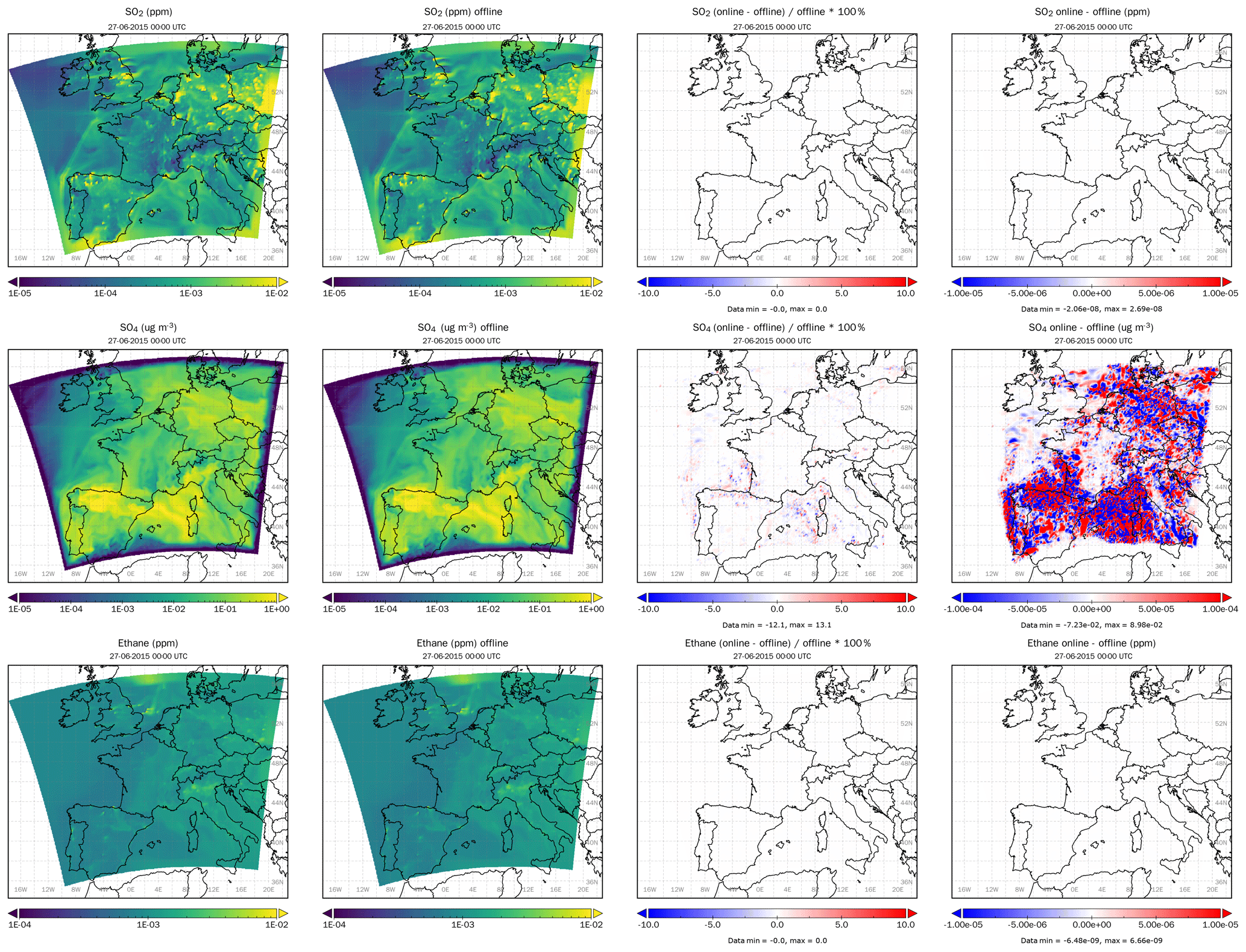
Figure 4Surface-layer concentrations for the online and offline simulations and relative and absolute differences between online and offline simulations in the COSMO-ART test case for surface layer fields of SO2 (top), SO4 (middle), and ethane (bottom) after 24 h.
Table 5Simulation time and input data size for online and offline COSMO-GHG and COSMO-ART test cases.
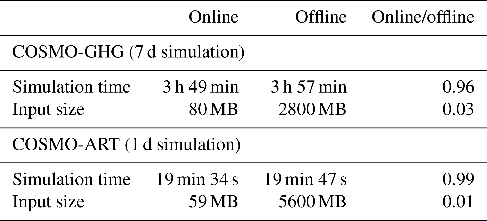
Table 6Benchmark for pre-processing online and offline emissions for the COSMO-GHG test case using the emiproc tool. Altogether, 19 categories from the emission inventories were processed (TNO: 14; Swiss: 5) as input for the CO2 tracer. Pre-processing was performed on a local Linux cluster, using 14 threads in parallel. Processing times for generating the mapping and country mask files are excluded. Results are shown for different dataset lengths.

A comprehensive online emission processing tool for atmospheric composition simulations was presented and demonstrated for two atmospheric transport models: COSMO-GHG and COSMO-ART. The tool is composed of a stand-alone Python package as well as a model-specific Fortran 90 module, which was integrated into the two models. The Python tool prepares the input for the simulation (a small set of netCDF files), which consists of gridded emission maps per source category (projected to the model grid), and temporal and vertical emission profiles. The Fortran 90 module reads these inputs at the beginning of a simulation and updates the 3D emissions for each simulated tracer at regular (e.g., hourly) intervals taking into account the corresponding temporal and vertical emission profiles. For COSMO-ART, additional speciation profiles have to be provided to distribute the emissions of a family of compounds like NMVOC over the individual model species.
The Python package is independent of the specific model implementation and is also able to generate hourly emission fields for models using the traditional offline approach. The Fortran 90 module, in contrast, was specifically designed for the two COSMO variants and will have to be adapted for other model systems.
The online approach greatly simplifies the setup of new model simulations, since a single set of a few input files is sufficient for all simulations on a given model grid irrespective of the simulated time period. In comparison to the offline approach, where a large number of emission input files has to be generated for a simulation, this reduces the input requirements by orders of magnitude.
The performance of the online and offline approaches was compared in two test simulations conducted with COSMO-GHG and COSMO-ART, respectively. In both cases the total computation time was almost identical, suggesting that the additional time required for computing hourly emissions online within the model could be compensated for by the reduced time spent on I/O. The time required for data pre-processing is much lower for the online approach. Both approaches produced almost identical concentration fields demonstrating their equivalence, with tiny differences attributable to floating point truncation errors.
The online emission approach was successfully introduced in all our COSMO-based model systems and, owing to its flexibility and reduced input and data pre-processing requirements, greatly simplified our daily working procedures. The Python package is a valuable tool on its own, as it is independent of the specific model system, can be applied in combination with several popular emission inventories, and offers an accurate mass-conserving method for mapping emissions to a given model grid.
Our tool is tailored to the processing of anthropogenic emissions, which follow a regular pattern in space and time, but it is not suitable for the processing of highly variable emissions such as emissions from biomass burning. This will require an extension to support a combination of offline inputs and online computation. Future developments will focus on the porting to other model systems such as ICON-ART and on the implementation of meteorology-dependent emissions such as those from residential heating or from lightning.
The Python package “emiproc” (Jähn et al., 2020) for emission pre-processing is publicly available through the C2SM GitHub organization (https://github.com/C2SM-RCM/cosmo-emission-processing, last access: 15 May 2020). The repository also includes the vertical and temporal profiles used here. The emission inventories are not part of the repository. The EDGAR inventory is accessible from the European Joint Research Centre (JRC). The TNO inventories can be accessed through the Copernicus product catalogue (https://atmosphere.copernicus.eu/catalogue, last access: 15 May 2020). The Swiss national emission inventories are available from the corresponding author upon request. The online emission module has been implemented both in COSMO-GHG and COSMO-ART. Both Fortran modules are available on the C2SM organization on GitHub and can be obtained from the corresponding author upon request. Access to the COSMO code is restricted to COSMO licensees. A free license can be obtained for research use following the procedure described at http://www.cosmo-model.org/content/consortium/licencing.htm, last access: 15 May 2020.
The supplement related to this article is available online at: https://doi.org/10.5194/gmd-13-2379-2020-supplement.
MJ led the writing of the paper with contributions from all co-authors and generated the figures. MJ, DO, GK, JMH, and QM jointly developed the Python package. VC, GK, DO, JMH, MJ, and KO jointly developed the Fortran modules. DB proposed the idea, surveyed the study, and contributed to the writing. QM and MJ conducted the COSMO-ART simulations and JMH the COSMO-GHG simulations.
The authors declare that they have no conflict of interest.
The work was also supported by a grant from the Swiss National Supercomputing Centre (CSCS) under project ID s862. Finally, we would like to acknowledge the contributions of Federal Office for Meteorology and Climatology MeteoSwiss, Swiss National Supercomputing Centre (CSCS), and ETH Zurich to the development of the GPU-accelerated version of COSMO.
This research has been supported by the following projects: SMARTCARB funded by the European Space Agency (ESA) under contract no. 4000119599/16/NL/FF/mg, CHE through the European Commission Horizon 2020 program under grant no. 776186, Carbosense4D funded by the Swiss Data Science Center, and Multiscale air pollution modeling funded by the Swiss Federal Office for the Environment.
This paper was edited by Augustin Colette and reviewed by two anonymous referees.
Athanasopoulou, E., Vogel, H., Vogel, B., Tsimpidi, A. P., Pandis, S. N., Knote, C., and Fountoukis, C.: Modeling the meteorological and chemical effects of secondary organic aerosols during an EUCAARI campaign, Atmos. Chem. Phys., 13, 625–645, https://doi.org/10.5194/acp-13-625-2013, 2013. a
Athanasopoulou, E., Speyer, O., Brunner, D., Vogel, H., Vogel, B., Mihalopoulos, N., and Gerasopoulos, E.: Changes in domestic heating fuel use in Greece: effects on atmospheric chemistry and radiation, Atmos. Chem. Phys., 17, 10597–10618, https://doi.org/10.5194/acp-17-10597-2017, 2017. a
Baklanov, A., Schlünzen, K., Suppan, P., Baldasano, J., Brunner, D., Aksoyoglu, S., Carmichael, G., Douros, J., Flemming, J., Forkel, R., Galmarini, S., Gauss, M., Grell, G., Hirtl, M., Joffre, S., Jorba, O., Kaas, E., Kaasik, M., Kallos, G., Kong, X., Korsholm, U., Kurganskiy, A., Kushta, J., Lohmann, U., Mahura, A., Manders-Groot, A., Maurizi, A., Moussiopoulos, N., Rao, S. T., Savage, N., Seigneur, C., Sokhi, R. S., Solazzo, E., Solomos, S., Sørensen, B., Tsegas, G., Vignati, E., Vogel, B., and Zhang, Y.: Online coupled regional meteorology chemistry models in Europe: current status and prospects, Atmos. Chem. Phys., 14, 317–398, https://doi.org/10.5194/acp-14-317-2014, 2014. a
Baldauf, M., Seifert, A., Forstner, J., Majewski, D., Raschendorfer, M., and Reinhardt, T.: Operational convective-scale numerical weather prediction with the COSMO model: description and sensitivities, Mon. Weather Rev., 139, 3887–3905, https://doi.org/10.1175/Mwr-D-10-05013.1, 2011. a
Bieser, J., Aulinger, A., Matthias, V., Quante, M., and Builtjes, P.: SMOKE for Europe – adaptation, modification and evaluation of a comprehensive emission model for Europe, Geosci. Model Dev., 4, 47–68, https://doi.org/10.5194/gmd-4-47-2011, 2011a. a
Bieser, J., Aulinger, A., Matthias, V., Quante, M., and van Der Gon, H. D.: Vertical emission profiles for Europe based on plume rise calculations, Environ. Pollut., 159, 2935–2946, https://doi.org/10.1016/j.envpol.2011.04.030, 2011b. a
Borge, R., Lumbreras, J., and Rodríguez, E.: Development of a high-resolution emission inventory for Spain using the SMOKE modelling system: A case study for the years 2000 and 2010, Environ. Model. Softw., 23, 1026–1044, https://doi.org/10.1016/j.envsoft.2007.11.002, 2008. a
Brunner, D., Kuhlmann, G., Marshall, J., Clément, V., Fuhrer, O., Broquet, G., Löscher, A., and Meijer, Y.: Accounting for the vertical distribution of emissions in atmospheric CO2 simulations, Atmos. Chem. Phys., 19, 4541–4559, https://doi.org/10.5194/acp-19-4541-2019, 2019. a, b, c
Centre on Emission Inventories and Projections (CEIP): User guide to WebDab, available at: https://www.ceip.at/ms/ceip_home1/ceip_home/webdab_emepdatabase/webdab_usersguide/ (last access: 10 July 2019), 2018. a
Crippa, M., Guizzardi, D., Muntean, M., Schaaf, E., Dentener, F., van Aardenne, J. A., Monni, S., Doering, U., Olivier, J. G. J., Pagliari, V., and Janssens-Maenhout, G.: Gridded emissions of air pollutants for the period 1970–2012 within EDGAR v4.3.2, Earth Syst. Sci. Data, 10, 1987–2013, https://doi.org/10.5194/essd-10-1987-2018, 2018. a
Denier van der Gon, H., Hendriks, C., Kuenen, J., Segers, A., and Visschedijk, A.: Description of current temporal emission patterns and sensitivity of predicted AQ for temporal emission patterns: TNO Report, EU FP7 MACC deliverable report D_D-EMIS_1.3, Report, MEP-R2003/166, Apeldoorn, The Netherlands, 2011. a
EEA: EMEP/CORINAIR Atmospheric emission inventory guidebook, 2nd Edn. 1999, Report, available at: https://www.eea.europa.eu/publications/EMEPCORINAIR/ (last access: 15 May 2020), 2000. a
Emmons, L. K., Walters, S., Hess, P. G., Lamarque, J.-F., Pfister, G. G., Fillmore, D., Granier, C., Guenther, A., Kinnison, D., Laepple, T., Orlando, J., Tie, X., Tyndall, G., Wiedinmyer, C., Baughcum, S. L., and Kloster, S.: Description and evaluation of the Model for Ozone and Related chemical Tracers, version 4 (MOZART-4), Geosci. Model Dev., 3, 43–67, https://doi.org/10.5194/gmd-3-43-2010, 2010. a
Freitas, S. R., Longo, K. M., Alonso, M. F., Pirre, M., Marecal, V., Grell, G., Stockler, R., Mello, R. F., and Sánchez Gácita, M.: PREP-CHEM-SRC – 1.0: a preprocessor of trace gas and aerosol emission fields for regional and global atmospheric chemistry models, Geosci. Model Dev., 4, 419–433, https://doi.org/10.5194/gmd-4-419-2011, 2011. a
Fuhrer, O., Osuna, C., Lapillonne, X., Gysi, T., Cumming, B., Bianco, M., Arteaga, A., and Schulthess, T.: Towards a performance portable, architecture agnostic implementation strategy for weather and climate models, Supercomput. Front. Innov. Int. J., 1, 45–62, https://doi.org/10.14529/jsfi140103, 2014. a
Glassmeier, F., Possner, A., Vogel, B., Vogel, H., and Lohmann, U.: A comparison of two chemistry and aerosol schemes on the regional scale and the resulting impact on radiative properties and liquid- and ice-phase aerosol–cloud interactions, Atmos. Chem. Phys., 17, 8651–8680, https://doi.org/10.5194/acp-17-8651-2017, 2017. a
Granier, C., Darras, S., Denier van der Gon, H., Doubalova, J., Elguindi, N., Galle, B., Gauss, M., Guevara, M., Jalkanen, J.-P., Kuenen, J., Liousse, C., Quack, B., Simpson, D., and Sindelarova, K.: The Copernicus Atmosphere Monitoring Service global and regional emissions (April 2019 version), https://doi.org/10.24380/D0BN-KX16, 2019. a
Guevara, M., Tena, C., Porquet, M., Jorba, O., and Pérez García-Pando, C.: HERMESv3, a stand-alone multi-scale atmospheric emission modelling framework – Part 1: global and regional module, Geosci. Model Dev., 12, 1885–1907, https://doi.org/10.5194/gmd-12-1885-2019, 2019. a
Jähn, M., Kuhlmann, G., Mu, Q., Haussaire, J.-M., Ochsner, D., and Brunner, D.: COSMO Emission Processing, Zenodo, https://doi.org/10.5281/zenodo.3760820, 2020. a
Janssens-Maenhout, G., Crippa, M., Guizzardi, D., Muntean, M., Schaaf, E., Dentener, F., Bergamaschi, P., Pagliari, V., Olivier, J. G. J., Peters, J. A. H. W., van Aardenne, J. A., Monni, S., Doering, U., and Petrescu, A. M. R.: EDGAR v4.3.2 Global Atlas of the three major Greenhouse Gas Emissions for the period 1970–2012, Earth Syst. Sci. Data Discuss., https://doi.org/10.5194/essd-2017-79, 2017. a
Keller, C. A., Long, M. S., Yantosca, R. M., Da Silva, A. M., Pawson, S., and Jacob, D. J.: HEMCO v1.0: a versatile, ESMF-compliant component for calculating emissions in atmospheric models, Geosci. Model Dev., 7, 1409–1417, https://doi.org/10.5194/gmd-7-1409-2014, 2014. a
Knote, C., Brunner, D., Vogel, H., Allan, J., Asmi, A., Äijälä, M., Carbone, S., van der Gon, H. D., Jimenez, J. L., Kiendler-Scharr, A., Mohr, C., Poulain, L., Prévôt, A. S. H., Swietlicki, E., and Vogel, B.: Towards an online-coupled chemistry-climate model: evaluation of trace gases and aerosols in COSMO-ART, Geosci. Model Dev., 4, 1077–1102, https://doi.org/10.5194/gmd-4-1077-2011, 2011. a, b
Kuenen, J. J. P., Visschedijk, A. J. H., Jozwicka, M., and Denier van der Gon, H. A. C.: TNO-MACC_II emission inventory; a multi-year (2003–2009) consistent high-resolution European emission inventory for air quality modelling, Atmos. Chem. Phys., 14, 10963–10976, https://doi.org/10.5194/acp-14-10963-2014, 2014. a, b
Lapillonne, X. and Fuhrer, O.: Using Compiler Directives to Port Large Scientific Applications to GPUs: An Example from Atmospheric Science, Parallel Processing Letters, 24, 1450003, https://doi.org/10.1142/S0129626414500030, 2014. a
Liu, Y., Gruber, N., and Brunner, D.: Spatiotemporal patterns of the fossil-fuel CO2 signal in central Europe: results from a high-resolution atmospheric transport model, Atmos. Chem. Phys., 17, 14145–14169, https://doi.org/10.5194/acp-17-14145-2017, 2017. a, b, c
Mailler, S., Menut, L., Khvorostyanov, D., Valari, M., Couvidat, F., Siour, G., Turquety, S., Briant, R., Tuccella, P., Bessagnet, B., Colette, A., Létinois, L., Markakis, K., and Meleux, F.: CHIMERE-2017: from urban to hemispheric chemistry-transport modeling, Geosci. Model Dev., 10, 2397–2423, https://doi.org/10.5194/gmd-10-2397-2017, 2017. a
Matthias, V., Arndt, J. A., Aulinger, A., Bieser, J., van der Gon, H. D., Kranenburg, R., Kuenen, J., Neumann, D., Pouliot, G., and Quante, M.: Modeling emissions for three-dimensional atmospheric chemistry transport models, J. Air Waste Manage., 68, 763–800, https://doi.org/10.1080/10962247.2018.1424057, 2018. a, b
McHenry, J. N., Ryan, W. F., Seaman, N. L., Coats, C. J., Pudykiewicz, J., Arunachalam, S., and Vukovich, J. M.: A Real-Time Eulerian Photochemical Model Forecast System: Overview and Initial Ozone Forecast Performance in the Northeast U.S. Corridor, B. Am. Meteorol. Soc., 85, 525–548, https://doi.org/10.1175/BAMS-85-4-525, 2004. a
Pouliot, G., Pierce, T., van der Gon, H. D., Schaap, M., Moran, M., and Nopmongcol, U.: Comparing emission inventories and model-ready emission datasets between Europe and North America for the AQMEII project, Atmos. Environ., 53, 4–14, https://doi.org/10.1016/j.atmosenv.2011.12.041, 2012. a
Roches, A. and Fuhrer, O.: Tracer module in the COSMO model, COSMO Technical Report, Report, 2012. a
Schindlbacher, S., Wankmüller, R., and Mareckova, K.: Best practice in gridding emissions – available tools, available at: https://tfeip-secretariat.org/assets/Meetings/Presentations/Zagreb-2016/Gridding.pdf (last access: 10 July 2019), 2016. a
Stockwell, W. R., Middleton, P., and Chang, J. S.: The second generation regional acid deposition model chemical mechanism for regional air quality modelling, J. Geophys. Res., 95, 16343–16367, 1990. a
Super, I., Dellaert, S. N. C., Visschedijk, A. J. H., and Denier van der Gon, H. A. C.: Uncertainty analysis of a European high-resolution emission inventory of CO2 and CO to support inverse modelling and network design, Atmos. Chem. Phys., 20, 1795–1816, https://doi.org/10.5194/acp-20-1795-2020, 2020. a
United Nations Economic Commission for Europe: Guidelines for Estimating and Reporting Emission Data under the Convention on Long-Range Transboundary Air Pollution, 65 pp., available at: http://digitallibrary.un.org/record/517855 (last access: 15 May 2020), Geneva, 2003. a
United Nations Economic Commission for Europe: Guidelines for reporting emissions and projections data under the Convention on Long-range Transboundary Air Pollution, available at: https://www.unece.org/fileadmin/DAM/env/documents/2015/AIR/EB/English.pdf (last access: 10 July 2019), 2015. a
Vogel, B., Vogel, H., Bäumer, D., Bangert, M., Lundgren, K., Rinke, R., and Stanelle, T.: The comprehensive model system COSMO-ART – Radiative impact of aerosol on the state of the atmosphere on the regional scale, Atmos. Chem. Phys., 9, 8661–8680, https://doi.org/10.5194/acp-9-8661-2009, 2009. a, b, c
Wang, S., Zheng, J., Fu, F., Yin, S., and Zhong, L.: Development of an emission processing system for the Pearl River Delta Regional air quality modeling using the SMOKE model: Methodology and evaluation, Atmos. Environ., 45, 5079–5089, https://doi.org/10.1016/j.atmosenv.2011.06.037, 2011. a
Weimer, M., Schröter, J., Eckstein, J., Deetz, K., Neumaier, M., Fischbeck, G., Hu, L., Millet, D. B., Rieger, D., Vogel, H., Vogel, B., Reddmann, T., Kirner, O., Ruhnke, R., and Braesicke, P.: An emission module for ICON-ART 2.0: implementation and simulations of acetone, Geosci. Model Dev., 10, 2471–2494, https://doi.org/10.5194/gmd-10-2471-2017, 2017. a
Wong, D. C., Pleim, J., Mathur, R., Binkowski, F., Otte, T., Gilliam, R., Pouliot, G., Xiu, A., Young, J. O., and Kang, D.: WRF-CMAQ two-way coupled system with aerosol feedback: software development and preliminary results, Geosci. Model Dev., 5, 299–312, https://doi.org/10.5194/gmd-5-299-2012, 2012. a
This is due to the fact that offline emissions are later pre-processed through int2lm, which requires a slightly larger domain.