2.1 Biases in FAMOUS

M16 speculated that both local climate biases and missing or incorrect processes in the land surface model – such as missing deep rooting in the Amazon – might be the cause of the simulated low forest fraction in the Amazon region at the end of the pre-industrial period in an ensemble of the climate model FAMOUS. In this study, we use the ensemble of FAMOUS previously used in M16, to attempt to find and correct the cause of persistent low forest fraction in the Amazon, identified in that paper.

FAMOUS (Jones et al., 2005; Smith et al., 2008) is a reduced-resolution climate simulator based on the HadCM3 climate model (Gordon et al., 2000; Pope et al., 2000). The model has many features of modern climate simulators but is of sufficiently low resolution to provide fast and simple data sets with which to develop UQ methods. Full details of the ensemble can be found in M16 and Williams et al. (2013).

The ensemble of 100 members perturbed seven land surface and vegetation inputs (see Table S1 in the Supplement), along with a further parameter denoted “beta” (β). Each of the 10 values of beta provides an index to 1 of 10 of the best-performing atmospheric and oceanic parameter sets used in a previous ensemble with the same model Gregoire et al. (2010), with the lowest values of beta corresponding to the very best performing variants. The beta parameter therefore summarised perturbations in 10 atmospheric and oceanic parameters that impacted the climate of the model randomly varied with land surface input parameters and potentially led to different climatologies in a model variant with the same land surface parameters but different values of beta. Variations in the beta parameter, however, did not correlate strongly to variations with any of the oceanic, atmospheric or land surface parameters in the ensemble, and so the parameter was excluded from the analysis in M16. In this analysis, we recognise that the different model climates caused by variations in the atmospheric and oceanic parameters will have an impact on the forest fraction, and so we summarise those variations directly using local temperature and precipitation.

Variation in the parameters across the ensemble had a strong impact on vegetation cover at the end of a spinup period, with atmospheric CO₂ at pre-industrial conditions. The broadleaf forest fraction in individual ensemble members varies from almost non-existent to vigorous (Fig. 1). The strong relationships between the global mean forest fraction and the mean forest fraction in each region imply that perturbations in input parameters exert a larger control over all forests simultaneously and individual forests to a smaller extent.

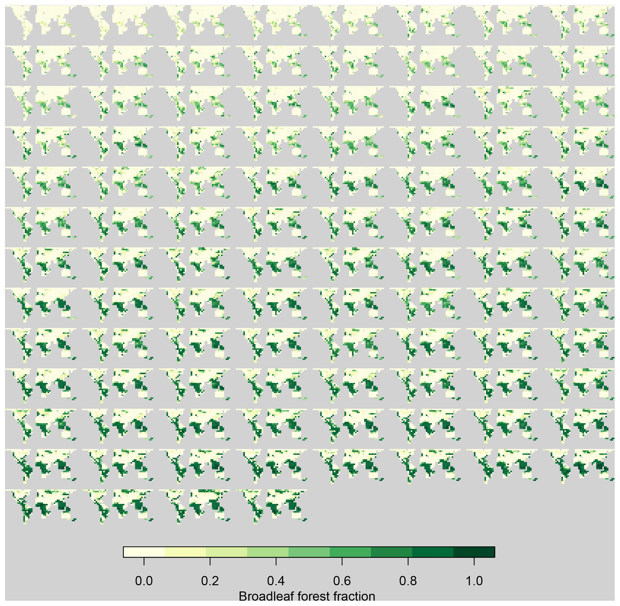
Figure 1Broadleaf forest fraction in the FAMOUS ensemble, ranked from the smallest to largest global mean value.

M16 aggregated the regional mean forest fraction for the Amazon, southeast Asian, North American and central African forests, along with the global mean. They were only able to find very few land surface parameter settings which the history matching process suggested should lead to an adequate simulations of the Amazon forests and the other forests together. These parameter sets were at the edges of sampled parameter space, where larger uncertainty in the emulator may have been driving the acceptance of the parameter sets.

In this study, we use the same ensemble of forest fraction data used in M16. However, we add temperature and precipitation data, present in the original ensemble but not used to build an emulator in the M16 study, to further our understanding of the causes of the low forest fraction in the Amazon region. The temperature and precipitation data summarise the effects of atmospheric parameters on the atmospheric component of the model, in a way that is directly seen by the land surface component of the model. We consider only regions dominated by tropical broadleaf forest, so as not to confound analysis by including other forests which may have a different set of responses to perturbations in parameters, rainfall and temperature.

For temperature observations, we use the Climate Research Unit (CRU) global monthly surface temperature climatology (Jones et al., 1999), covering the years 1960–1990. For precipitation, we use the average monthly rate of precipitation, covering the years from 1979 to 2001 from the Global Precipitation Climatology Project (GPCP) version 2.2, provided by the NOAA/OAR/ESRL PSD, Boulder, Colorado, USA, from their website at https://www.esrl.noaa.gov/psd/ (last access: 22 October 2014) (Adler et al., 2003). Vegetation fraction observations are adapted from Loveland et al. (2000) and are shown in Fig. 2. Although the observations all cover slightly different time periods, we expect the differences caused by harmonising the time periods to be very small compared to other uncertainties in our analysis and to be well covered by our uncertainty estimates.

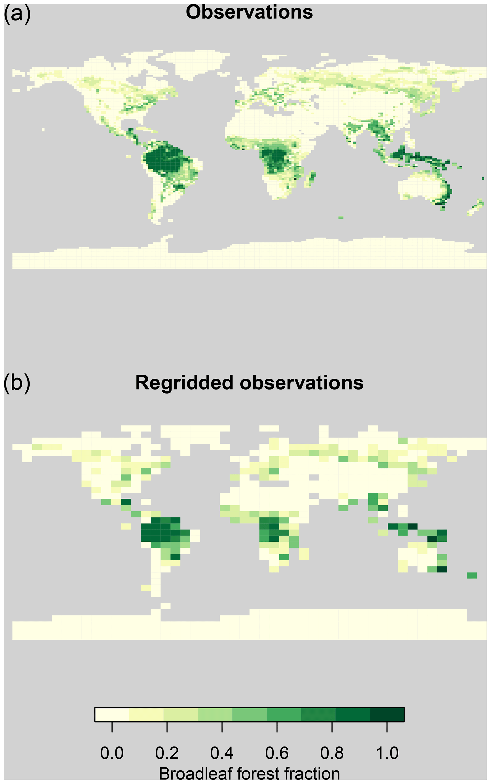
Figure 2Observations of broadleaf forest fraction on their native grid (a) and regridded to the FAMOUS grid (b).

A plot of regional mean temperature and precipitation in the tropical forest regions in the FAMOUS ensemble (Fig. 3) indicates the form of the impact that the regional climate has on forest fraction in the climate model. Central African and southeast Asian climates in the model simulations run in a sweep across the middle of the plot, from dry and cool to wet and warm.

It appears that a wetter climate – which would be expected to stabilise forests – broadly compensates for the forest reductions induced by a warmer climate. Within the ensemble of central African forests, for example, forest fraction increases towards the “cooler, wetter” (top left) part of the climate phase space. Beyond a certain value, however, there are no simulated climates or forests in this climatic region. It is clear from the plot that while central African and southeast Asian forests are simulated in the large part considerably warmer than recent observations, they are also simulated considerably wetter, which might be expected to compensate forest stability. In contrast, while simulated considerably warmer, the Amazon is also slightly drier than recent observations, which might further reduce forest stability.

Figure 3Regional temperature, precipitation and broadleaf forest fraction in the ensemble of FAMOUS compared with observations. Smaller symbols represent broadleaf forest fraction in the FAMOUS ensemble against regional mean temperature and precipitation. Ensemble member forest fraction in the Amazon is represented by the colour of the circles, central Africa by triangles and SE Asia by squares. Larger symbols represent observed climate and forest fraction.

Download

We are assuming here that tropical forests can be represented by a single set of forest function parameters. While such an assumption risks missing important differences across heterogenous tropical forests, modelling the system with the smallest set of common parameters avoids overfitting to present-day data. Avoiding overfitting is important if we are to use these models to project forest functioning in future climates outside observed conditions. One of the questions that the analysis presented in this paper addresses is whether current forest biases in the simulations reflect limitations of this single tropical forest assumption or whether biases in the simulations of the wider climate variables play a more important role.

3.1 An augmented emulator

Our strategy is to augment the design matrix of input parameters X with corresponding atmospheric climate model output that might have an impact on the modelled land surface, building an emulator that models the effects of both input parameters and climate on forest fraction. We then use the augmented emulator to bias correct each forest in turn. We use the emulator to describe the relationship between land surface parameters, atmospheric variables that summarise the action of hidden atmospheric parameters and the broadleaf forest fraction. The relationships between these variables are summarised in Fig. 4.

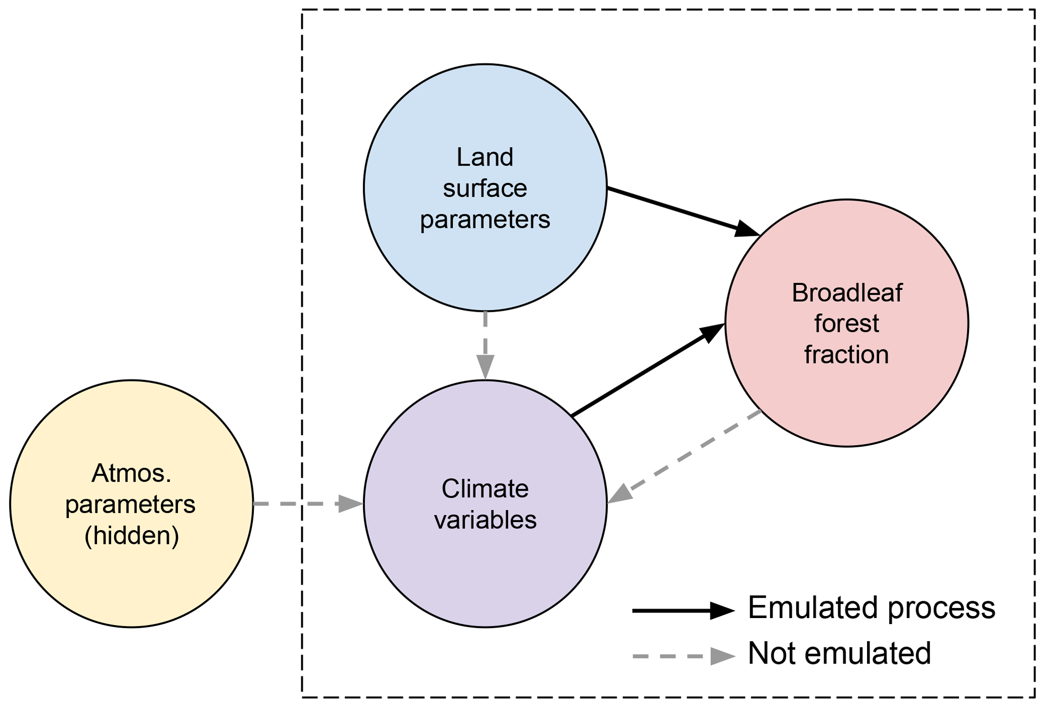
Figure 4A graph showing the assumed relationship between input parameters, climate variables and forest fraction. An arrow indicates influence in the direction of the arrow. Processes that are directly emulated are shown with a solid arrow, while the processes shown by a dotted arrow are not directly emulated.

Download

We have a number of forests for each ensemble member, differing in driving influence by a different local climate. Regional extent of each of the broadleaf forests can be found in the Supplement. We use regional mean temperature (T) and precipitation (P) for each of the forests: the Amazon, central Africa and southeast Asia as additional inputs to augment our original design matrix of land surface parameters, X. These new inputs are outputs of the model when run at the original inputs X and are influenced by the 10 atmospheric and oceanic parameters perturbed in a previous ensemble in a configuration unavailable to us in this experiment. Performance of the model under those perturbations is summarised in the beta parameter, which has smaller values for the better-performing models. The performance metrics included temperature and precipitation, along with a number of other measures, so the beta parameter therefore contains information about temperature and precipitation across the ensemble, without being a perfect representation of its behaviour. We cannot control the atmospheric and oceanic parameters directly and thus ensure that they lie in a Latin hypercube configuration, although the ensemble is ordered in a Latin hypercube configuration according to the performance of the model at each parameter set.

With n=100 ensemble members, we form each n×1 vector of temperature and precipitation and form an n×2 matrix of climate variables for the Amazon C_AZ=[T_AZP_AZ], central Africa C_AF=[T_AFP_AF] and southeast Asia C_AS=[T_ASP_AS]. We use these to augment the original n×p input matrix X, creating a unique input location for each forest. We then stack these augmented input matrices together to form a single input matrix X^′.

From an initial ensemble design matrix with n=100 members and p=7 inputs, we now have a design with n=300 members and p=9 inputs. Each member with a replicated set of initial input parameters (e.g. members $[\mathrm{1},\mathrm{101},\mathrm{201}]$), differs only in the T and P values. Figure 5 shows a diagram of the augmented emulator along with the composition of the resulting input matrix and output vector.

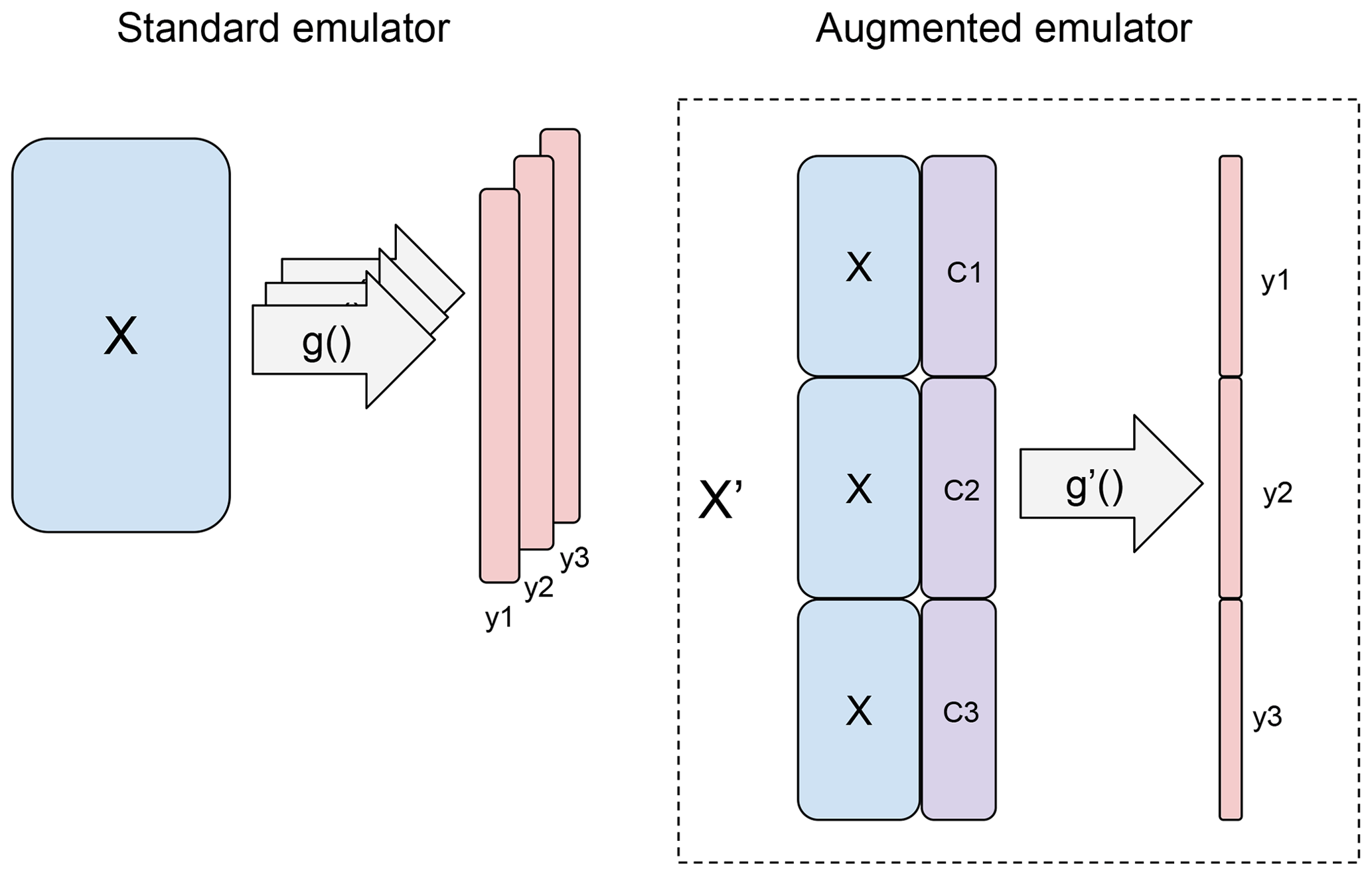
Figure 5In a standard emulator setup (left), training data consist of an input matrix X and corresponding simulator output y. A new emulator $g_{\mathrm{1}}\left(\right),\mathrm{\dots },g_{\mathrm{3}}\left(\right)$ is trained for each output ${\mathit{y}}_{\mathrm{1}},\mathrm{\dots },{\mathit{y}}_{\mathrm{3}}$ of interest. In the augmented emulator, output from the simulator ${\mathbf{C}}_{\mathrm{1}},\mathrm{\dots },{\mathbf{C}}_{\mathrm{3}}$ augments the design matrix, with the initial inputs X repeated.

Download

Where in M16, the authors built an independent emulator for each output (i.e. regional forest fraction), we now build a single emulator for all forest fractions simultaneously given input parameters, temperature and precipitation. The output vector for the tropical forests has gone from being three sets of 100 values y_AZ, y_AF, y_AS, to a single vector ${\mathit{y}}^{\mathbf{\prime }}=[{\mathit{y}}_{\mathrm{AZ}},{\mathit{y}}_{\text{AF}},{\mathit{y}}_{\text{AS}}]$ of length 300. We model forest fraction y^′ as a function of X^′ using the Gaussian process emulator of the DiceKriging package (Roustant et al., 2012) in the R statistical language and environment for statistical computing. Details of the emulator can be found in the Supplement.

We note that the augmented emulator depends on the assumption that modelled broadleaf forests in each location respond similarly to perturbations in climate and input parameters. This assumption may not hold for the behaviour of the forests in the model or indeed the real world. For example, particularly deep rooting of forests in the Amazon would respond differently to rainfall reductions but these processes are not represented in the underlying climate model. Similarly, differing local topology that is captured in the climate model may influence the forests in a way not captured by our emulator. In both cases, the emulator would show systematic errors of prediction.

3.2 Verifying the augmented emulator

To verify that the augmented emulator adequately reproduces the simulator behaviour, we use a leave-one-out metric. For this metric, we sequentially remove one simulator run from the ensemble, train the emulator on the remaining ensemble members and predict the held-out run. We present the predicted members and the calculated uncertainty plotted against the actual ensemble values in Fig. 6.

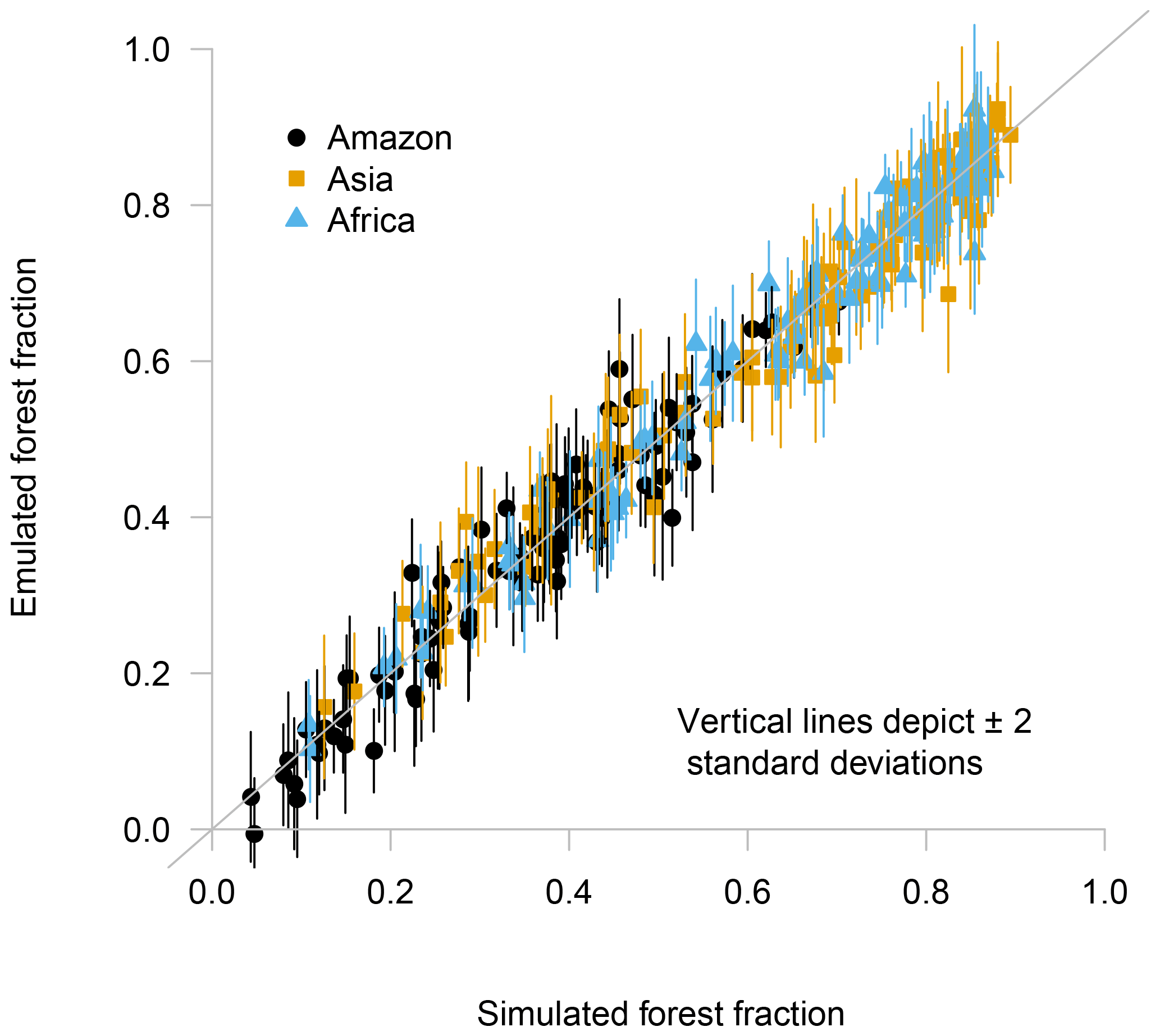
Figure 6Leave-one-out cross-validation plot, with the true value of the simulator output on the x axis and predicted output on the y axis. Vertical lines indicate ±2 standard deviations.

Download

It is important to check that the augmented emulator performs well in prediction, in order to have confidence that using emulated runs in our later analyses is a valid strategy. We see no reason to doubt that the augmented emulator provides a good prediction and accurate uncertainty estimates for prediction at inputs points not yet run. We use the mean of the absolute value of the difference between the emulator prediction and corresponding held-out value to calculate the mean absolute error (MAE) of cross-validation prediction. Prediction error and uncertainty estimates remain approximately stationary across all tropical forests and values of forest fraction. The mean absolute error of prediction using this emulator is a little under 0.03 or around 6 % of the mean value of the ensemble.

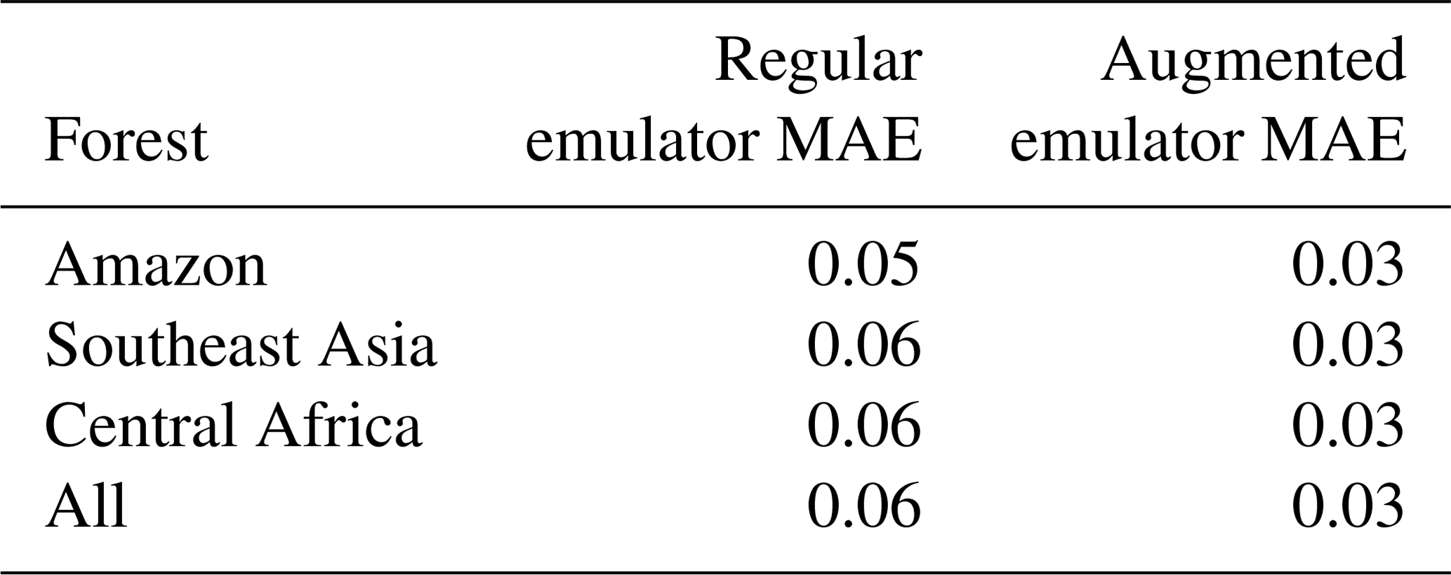
When compared against the regular emulator using just the land surface inputs, the augmented emulator performs well. The regular emulator built individually for each of the forests (as per M16) has a mean absolute error value of 0.058 – nearly double that of the augmented emulator. This indicates that adding temperature and precipitation to the input matrix adds useful information to a predictive statistical model. A breakdown of the mean absolute error of the emulator on a per-forest basis can be seen in Table 1.

There is some concern that the emulator might not perform well close to the observed values of temperature and precipitation, particularly for the Amazon and central African regions. For this reason, we carry out an enhanced verification of the emulator, holding out more ensemble members and demanding further extrapolation (see Sect. S2 in the Supplement). We find no reason to doubt that the augmented emulator performs well.

Table 1Mean absolute error (MAE) rounded to the first significant figure for the regular emulator, using just the seven land surface inputs, and the augmented emulator, including temperature and precipitation.

Download Print Version | Download XLSX

Do the error estimates of the augmented emulator match the true error distributions when tested in leave-one-out predictions? We test the reliability of uncertainty estimates of the emulator by checking that the estimated probability distributions for held-out ensemble members match the true error distributions in the leave-one-out exercise. We create a rank histogram (see, e.g. Hamill, 2001) for predictions, sampling 1000 times from each Gaussian prediction distribution and plotting the rank of the actual prediction in that distribution. The distribution of these ranks overall predictions should be uniform if the uncertainty estimates are reliable. Consistent overestimation of uncertainty will produce a peaked histogram, while systematic underestimation of uncertainty will produce a U-shaped histogram. The rank histogram produced by this set of predictions (Fig. 7) is close to a uniform distribution, indicating reliable predictions.

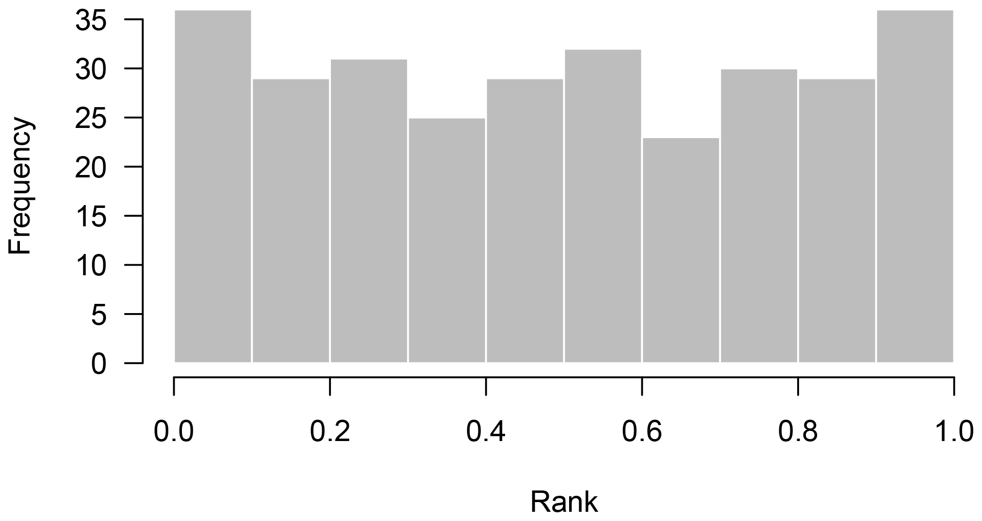
Figure 7Rank histogram of leave-one-out predictions. For each prediction of a held-out ensemble member, we sample 1000 points from the Gaussian prediction distribution and then record where the true held-out ensemble member ranks in that distribution. We plot a histogram of the ranks for all 300 ensemble members. A uniform distribution of ranks indicates that uncertainty estimates of the emulator are well calibrated.

Download

3.3 History matching

History matching is the process of finding and ruling out regions of parameter space where the model is unlikely to produce output that matches observations well. It measures the statistical distance between an observation of a real-world process and the emulated output of the climate model at any input setting. An input where the output is deemed too far from the observation is ruled “implausible” and removed from consideration. Remaining inputs are conditionally accepted as “not ruled out yet” (NROY), recognising that further information about the model or observations might yet rule them as implausible.

Observations of the system are denoted z, and we assume that they are made with uncorrelated and independent errors ϵ such that

Assuming a “best” set of inputs x^*, where the model discrepancy δ or difference between climate model output y and z is minimised, we relate observations to inputs with

We calculate measure of implausibility I and reject any input as implausible where I>3 after Pukelsheim's 3σ rule; that is, for any unimodal distribution, 95 % of the probability mass will be contained within 3 standard deviations of the mean (Pukelsheim, 1994). We calculate

which recognises that the distance between the best estimate of the emulator and the observations must be normalised by uncertainty in the emulator g(x) in the observational error ϵ and in the estimate of model discrepancy δ.

4.1 The joint impacts of temperature and precipitation on forest fraction

What impact do temperature and precipitation have on forest fraction together? We use the emulator from Sect. 3.1 and predict the simulator output across the entire range of simulated temperature and precipitation, while holding the other inputs at their default values. The marginal impacts of temperature and precipitation on forest fraction are clear in Fig. 8. Ensemble member temperature, precipitation and forest fraction, taken from Fig. 3, are overplotted for comparison. Temperature and precipitation values are normalised to the range of the ensemble in this plot.

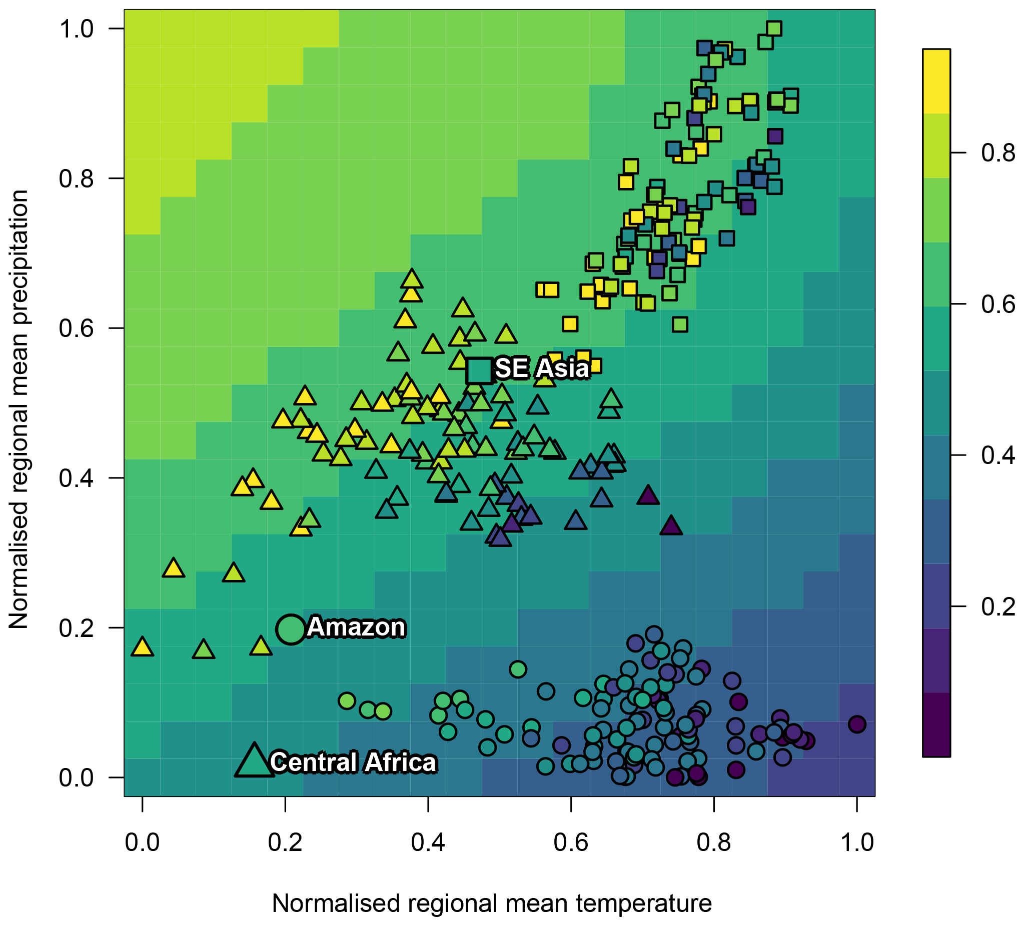
Figure 8The impact of climate on forest fraction. Background plot colour indicates the mean emulated forest fraction when all land surface inputs are held at their default values. Temperature and precipitation in the ensemble are marked with symbols, with the fill colour representing forest fraction. Larger symbols represent the values observed in the real world.

Download

With other inputs held constant, cooler, wetter climates are predicted to increase forest fraction and drier, warmer climates reduce forest fraction. In general, southeast Asian and central African forests are simulated as warmer and wetter than their true-life counterparts. Moving the temperature and precipitation values of a typical ensemble member from near the centre of these forest sub-ensembles to their observed real-world values would shift them primarily in the same direction as the contours of forest fraction value. This would mean that bias correcting the climate variables would not have a large impact on forest fraction values in southeast Asian and central African forests, and that they are therefore simulated with a roughly accurate forest fraction. In contrast, the Amazon is simulated slightly drier and considerably warmer than the observed Amazon and many ensemble members consequently have a lower forest fraction than observed. Shifting the temperature and precipitation of a typical ensemble member for the Amazon to its real-world observed values would cross a number of contours of forest fraction. This figure provides strong evidence that a significant fraction of the bias in Amazon forest fraction is caused by a bias in simulated climate.

4.2 A climate bias correction approach

With an emulator that models the relationship between input parameters, local climate and the forest fraction, we can predict what would happen to forest fraction in any model simulation if the local climate was correct. In Fig. 9, we compare the value of forest fraction predicted at the default set of land surface parameters using the standard emulator, with that predicted using the local temperature and precipitation corrected to the observed values using the augmented emulator. This means that central Africa becomes significantly drier and a little cooler than the centroid of the ensemble. Southeast Asia becomes a little cooler and a little drier. The Amazon forest becomes a little wetter and significantly cooler. The ensemble has a much larger spread of climates in central Africa than southeast Asia or the Amazon. We note that we do not have an ensemble member run at the default land surface parameters, so we compare two predictions using the emulator.

The bias correction reduces the difference between the prediction for the modelled and observed Amazon forest fraction markedly, from −0.28 using the standard emulator to −0.08 using the augmented emulator. It makes the predicted modelled forest in central Africa worse (−0.11 from −0.03) and slightly improves the SE Asian forest fraction (0.07 from 0.1). Overall, bias correcting the climate takes the mean absolute error at the default parameters from 0.14 to 0.09 for the three forests. It is possible that the predicted forest fraction for central Africa is slightly worse because the observed climate is towards the edge of the parameter space of temperature and precipitation, and there are no runs near.

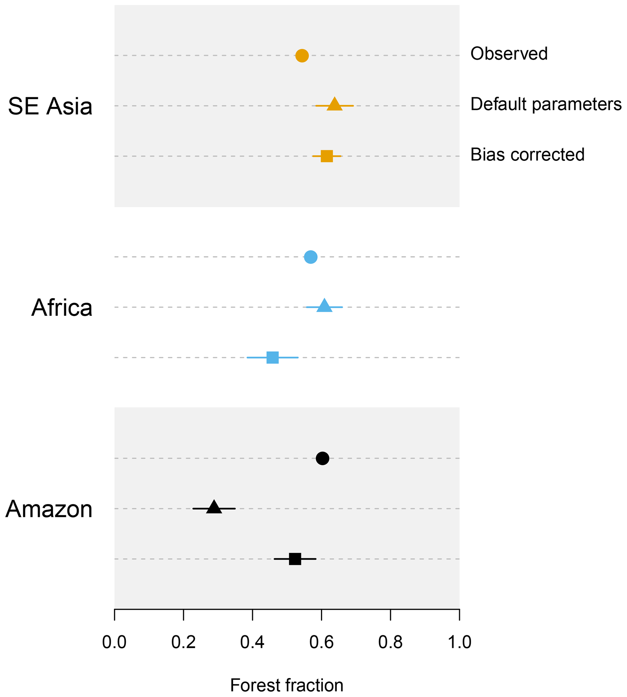
Figure 9Observed and emulated forest fraction in each tropical forest. For the emulated forest fraction at default and bias-corrected parameters, emulator uncertainty of ±2 SD is represented by horizontal bars.

Download

Table 2Mean absolute error of the simulated forest fraction and implausibility of the default set of land surface parameters when not bias corrected and bias corrected to temperature and precipitation observations.

Download Print Version | Download XLSX

4.3 History matching to learn about model discrepancy

In this section, we use history matching (see Sect. 3.3) to learn about parts of input parameter space that are consistent with observations and to find the causes of discrepancy in the model. We study the region of input space that is NROY by comparison of the model output to the observations of forest fraction. In the previous section, we see that the overall difference between the simulated and observed forest fraction is reduced if the output is bias corrected. In this section, we study how that bias correction affects the NROY space.

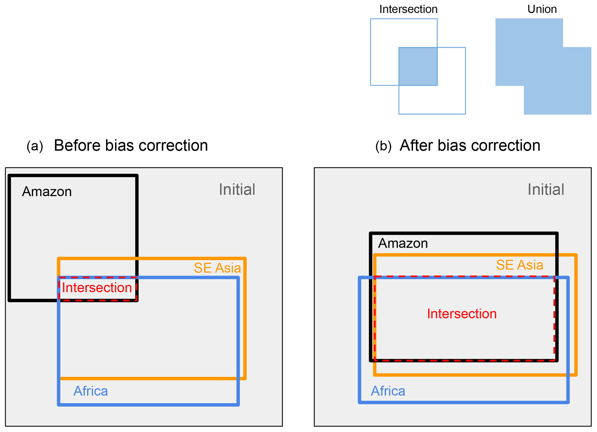
Figure 10A cartoon depicting the input space that is NROY when the climate simulator output is compared to observations of the forest fraction in the Amazon, Africa and southeast Asia before (a) and after (b) bias correction. We measure the “shared” space (the intersection of NROY spaces for each forest) as a fraction of the union (the total space covered by all three forests) of the NROY spaces. The “initial” space represents the total parameter space covered by the ensemble.

Download

In M16, the default input parameters were ruled out as implausible for the Amazon region forest fraction. For the sake of illustration, we assume very low uncertainties: zero observational uncertainty and a model discrepancy term with a zero mean and an uncertainty (±1 SD) of just 0.01. We note that under these conditions the default parameters would be ruled out in the standard emulator. However, if we bias correct the model output using the observed temperature and precipitation, we find that the implausibility measure I for the forest fraction in the Amazon at the standard input parameters reduces from nearly 7 to 1.3 – comfortably under the often-used threshold of 3 for rejection of an input. The implausibility of the SE Asian and central African forest fraction at the default parameter settings rises with bias correction (see Table 2), but neither comparison comes close to ruling out the default parameters. This rise in implausibility is caused by a smaller uncertainty estimate (in the case of SE Asia) and a larger emulation error (in the case of central Africa). However, we can confidently say that bias correction using the emulator means that observations no longer rule out the default parameters, even with the assumption of a very small model discrepancy.

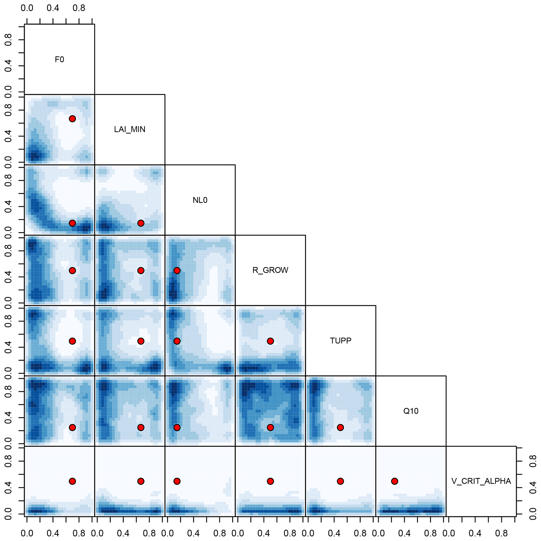
Figure 11NROY land surface input space shared by all three forests before bias correction. Blue shading denotes the density of NROY input candidates, projected into the two-dimensional space indicated by the labels. The default parameter settings are marked as red points.

Download

Another result of bias correction is that it increases the “harmonisation” of the input spaces – that is, the volume of the input space that is “shared” or NROY by any of the comparisons of the simulated forest fractions with data. In M16, we argued that the regions of input parameter space where the model output best matched the observations had a large shared volume for the central African, southeast Asian and North American forests. In contrast, the “best” input parameters for the Amazon showed very little overlap with these other forests. This pointed to a systematic difference between the Amazon and the other forests that might be a climate bias or a fundamental discrepancy in the land surface component of the model. Here, we show that the climate-bias-corrected forest in the Amazon would share a much larger proportion of its NROY space with the other forests. Indeed, the default parameters are now part of this “shared” space, and there is formally no need to invoke an unexplained model discrepancy in order to accept them for all the tropical forests. We show a cartoon of the situation in Fig. 10.

Table 3Measures of the NROY input space shared by all three forests. The intersection is NROY for all three forests, the union is NROY for at least one forest. The initial space is that defined by the parameter limits of the initial experiment design.

Download Print Version | Download XLSX

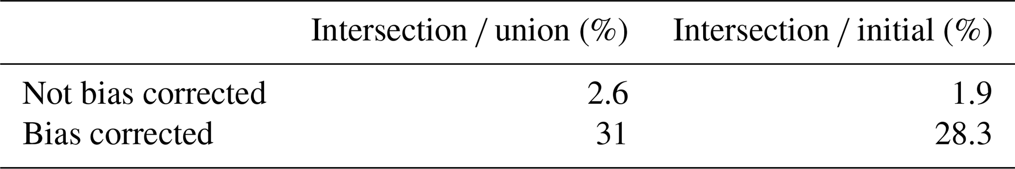
We find that when we bias correct all the spaces, the proportion of “shared” NROY input space relative to the union of NROY spaces for all forests increases from 2.6 % to 31 % – an order of magnitude increase (see Table 3). This is driven chiefly by the harmonisation of the NROY space of the Amazon to the other two forests. We see that before bias correction, the southeast Asian and African forests share nearly three quarters (74 %) of their combined NROY space. This drops to 33 % when bias corrected, but with the advantage that the Amazon and central Africa now share over 90 % (91.5 %) of their combined NROY space (Table 4).

When compared to the initial input parameter space covered by the ensemble, the shared NROY space of the non-bias-corrected forests represents 1.9 %, rising to 28 % on bias correction.

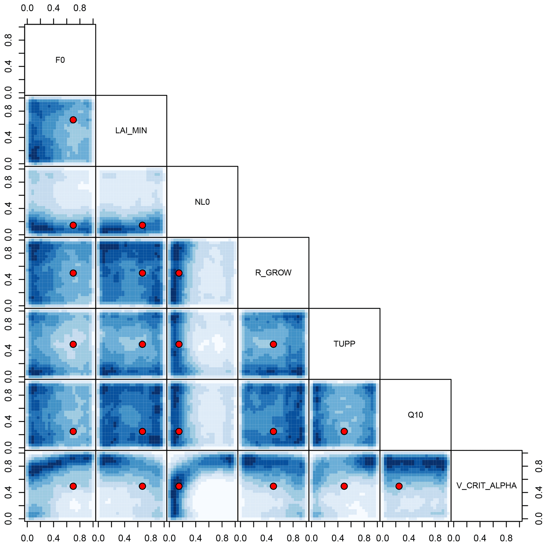
Figure 12NROY land surface input space shared by all three forests when bias corrected using the augmented emulator. Blue shading denotes the density of NROY input candidates, projected into the two-dimensional space indicated by the labels. The default parameter settings are marked as red points.

Download

We visualise two-dimensional projections of the NROY input parameter space shared by all three forests before bias correction in Fig. 11 and after bias correction in Fig. 12. The two-dimensional projections of high-density regions of NROY points are dramatically shifted and expanded in the bias-corrected input space, and the default parameters now lie in a high-density region. For example, a high-density region of NROY points is apparent in the bias-corrected input parameter space (Fig. 12), in the projection of V_CRIT_ALPHA and NL0. It is clear from sensitivity analyses (Sect. 4.4) that, all other things remaining the same, increasing the value of NL0 strongly raises forest fraction, while increasing V_CRIT_ALPHA strongly reduces forest fraction. We would expect there to be a region, indeed a plane through parameter space where these two strong effects counteract each other, resulting in a forest fraction close to observations. This feature does not appear in the history matching before bias correcting (Fig. 11). The low value of the simulated Amazon forest fraction before bias correction of the climate inputs rules out much of the input parameter space later found to be NROY after the bias-corrected history matching exercise (Fig. 12).

It is possible that the estimate of shared NROY input space is larger than it could be, due to the lack of ensemble runs in the “cool, wet” part of parameter space, where there are no tropical forests. Inputs sampled from this part of parameter space may not be ruled out, as the uncertainty on the emulator may be large. This is history matching working as it should, as we have not included evidence about what the climate model would do if run in this region. Further work could explore the merits of including information from other sources (for example, from our knowledge that tropical forests do not exist in a cool, wet climate) into the history matching process.

Table 4Proportion of shared NROY input space for each forest pair compared to the total NROY space covered by the same forest pair. Not bias corrected (top) and bias corrected (bottom).

Download Print Version | Download XLSX

4.4 Sensitivity analysis

The augmented emulator allows us to measure the sensitivity of forest fraction to the land surface input parameters simultaneously with climate variables temperature and precipitation. A quantitative measure of sensitivity of the model output to parameters that does take into account interactions with other parameters is found using the FAST99 algorithm of Saltelli et al. (1999), summarised in Fig. 13. Precipitation and temperature are the second and third most important parameters, more important than NL0, and only slightly less important than V_CRIT_ALPHA. Interaction terms contribute a small but non-negligible part to the sensitivity. This form of quantitative sensitivity analysis is useful to understand initial model behaviour but could be vulnerable to error, as it is assumed that all parts of the input space are valid. Our experiment design does not control temperature and precipitation directly, and the “cool, wet” part of this parameter space does not contain tropical broadleaf forest. It is possible therefore that a sensitivity analysis that relies on input samples from this region might mis-specify sensitivity indices. Below, we outline two methods that tackle this problem: one-at-a-time sensitivity analysis with history matching and Monte Carlo filtering.

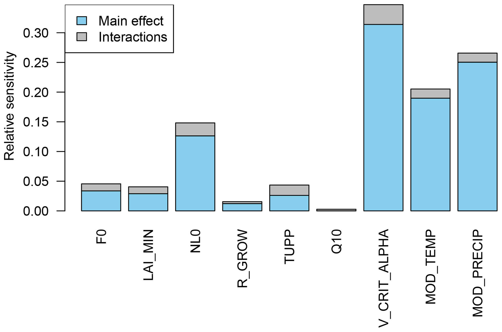
Figure 13Sensitivity of forest fraction to model parameters and climate parameters, found using the FAST99 algorithm of Saltelli et al. (1999).

Download

We measure the one-at-a-time sensitivity to parameters and climate variables, using the augmented emulator to predict changes in forest fraction as each input is changed from the lowest to highest setting in turn, with all other inputs at the default settings or observed values. We present the results in Fig. 14. In this diagram, we exclude emulated forests that are deemed implausible according to the criteria in Sect. 3.3. This is to avoid potentially overestimating the sensitivity of forest fraction to (for example) temperature and precipitation by including results from regions of parameter space far from existing ensemble members and in very different climate regimes from existing broadleaf tropical forests.

Parameters NL0 and V_CRIT_ALPHA and climate variables temperature and precipitation exert strong influence of similar magnitudes on forest fraction. Shaded regions represent the uncertainty of the sensitivity to each parameter, due to estimated emulator uncertainty of ±2 standard deviations. This sensitivity measure does not include the extra uncertainty due to the fact that the relationships will change depending on the position of the other parameters. We do, however, see a measure of how temperature and precipitation affect the marginal response of the other parameters, as the observed climates of each forest are different. For example, we clearly see that the response of the forest fraction to, e.g. NL0, depends on climate – the forest fraction response is a noticeably different shape when varied under the mean climate of the southeast Asian region.

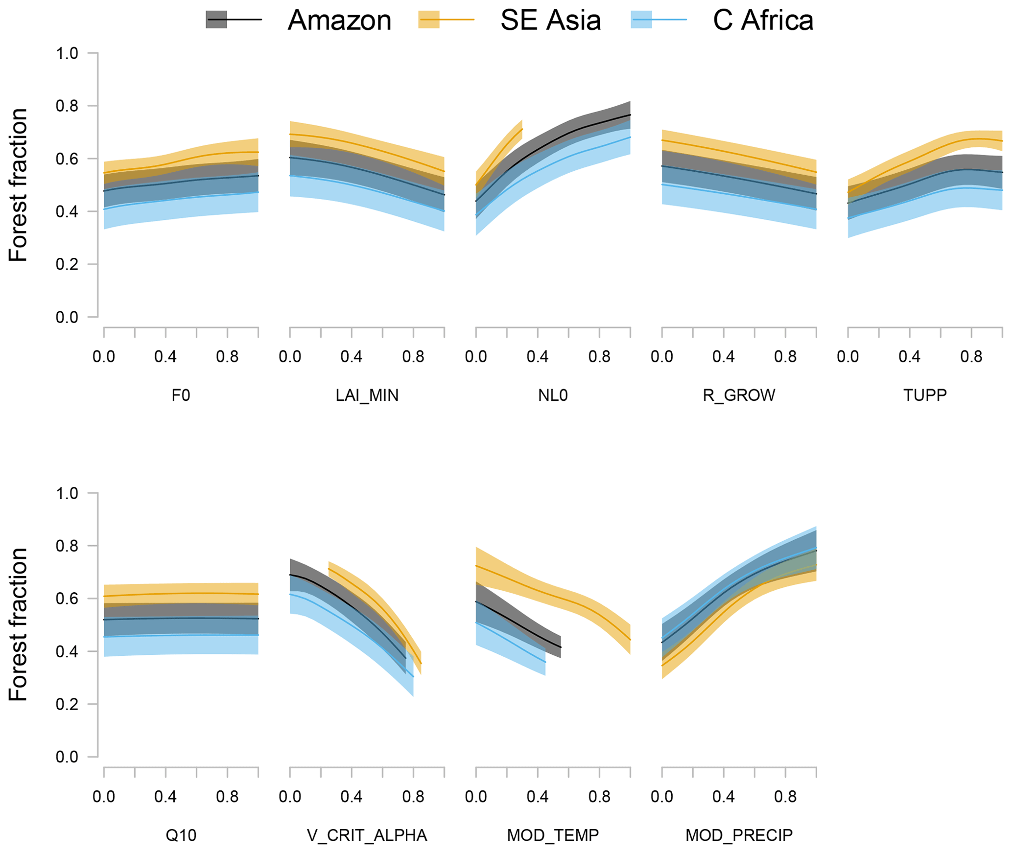
Figure 14One-at-a-time sensitivity of forest fraction variation of each parameter and climate variable in turn across the NROY parameter range. All other parameters or variables are held at their default values while each parameter is varied, and values of model broadleaf forest fraction which are statistically far from observations are excluded. Solid lines represent the emulator mean and shaded areas represent ±2 standard deviations of emulator uncertainty.

Download

A technique called Monte Carlo filtering (MCF), or regional sensitivity analysis, is useful in situations where input parameter distributions are non-uniform or correlated, or not all parts of parameter space are valid. The basic idea of MCF is to split samples from the input space into those where the corresponding model output meets (or not) some criteria of behaviour. Examining the differences between the cumulative distributions of those inputs where the outputs do or do not meet the criteria provides a measure of sensitivity of the output to that input. For example, we might split model behaviour into those outputs above or below a threshold. A recent description of MCF and references can be found in Sect. 3.4 of Pianosi et al. (2016).

We integrate the MCF sensitivity analysis into the history matching framework. We examine the differences in the univariate cumulative distributions of each parameter, in those samples where the output is ruled out by history matching, against those that are NROY. To measure the differences between the distributions, we perform a two-sided Kolmogorov–Smirnov (KS) test and use the KS statistic as in indicator that the output is sensitive to that input. A larger KS statistic indicates that the cumulative distribution functions of the respective inputs are further apart, that input is more important for determining if the output falls within the NROY part of parameter space, and therefore the output is more sensitive to that input in a critical region. We note that MCF is useful for ranking parameters but not for screening, as inputs that are important only in interactions might have the same NROY and ruled out marginal distributions. In this case, they would have a sensitivity index of zero.

We apply MCF using the emulator. This allows us to examine the difference between model output distributions given a much larger sample from the input space than when using only the ensemble. This comes at the cost of using an imperfect emulator, which may give different results than if we were using a large ensemble of runs. To avoid the problem of sampling precipitation and temperature from regions where there are no ensemble members, we sample uniformly from across input space for all other parameters and then append a random temperature/precipitation location from the ensemble. We calculate a sampling uncertainty by calculating the MCF sensitivity metrics 1000 times, each time using a sample size of 5000 emulated ensemble members. In this way, we estimate both the mean and the uncertainty (standard deviation) of the MCF sensitivity measures. We note that the sensitivity indices are calculated higher when a small number of ensemble members are used, as well as with a higher uncertainty. The change in both the estimated statistic and its uncertainty have begun to become small by the time 3000 ensemble members are used, suggesting that we should use at least this many emulated ensemble members to obtain an unbiased sensitivity analysis (see the Supplement). We compare the KS statistics and their associated uncertainty for each input in Fig. 15.

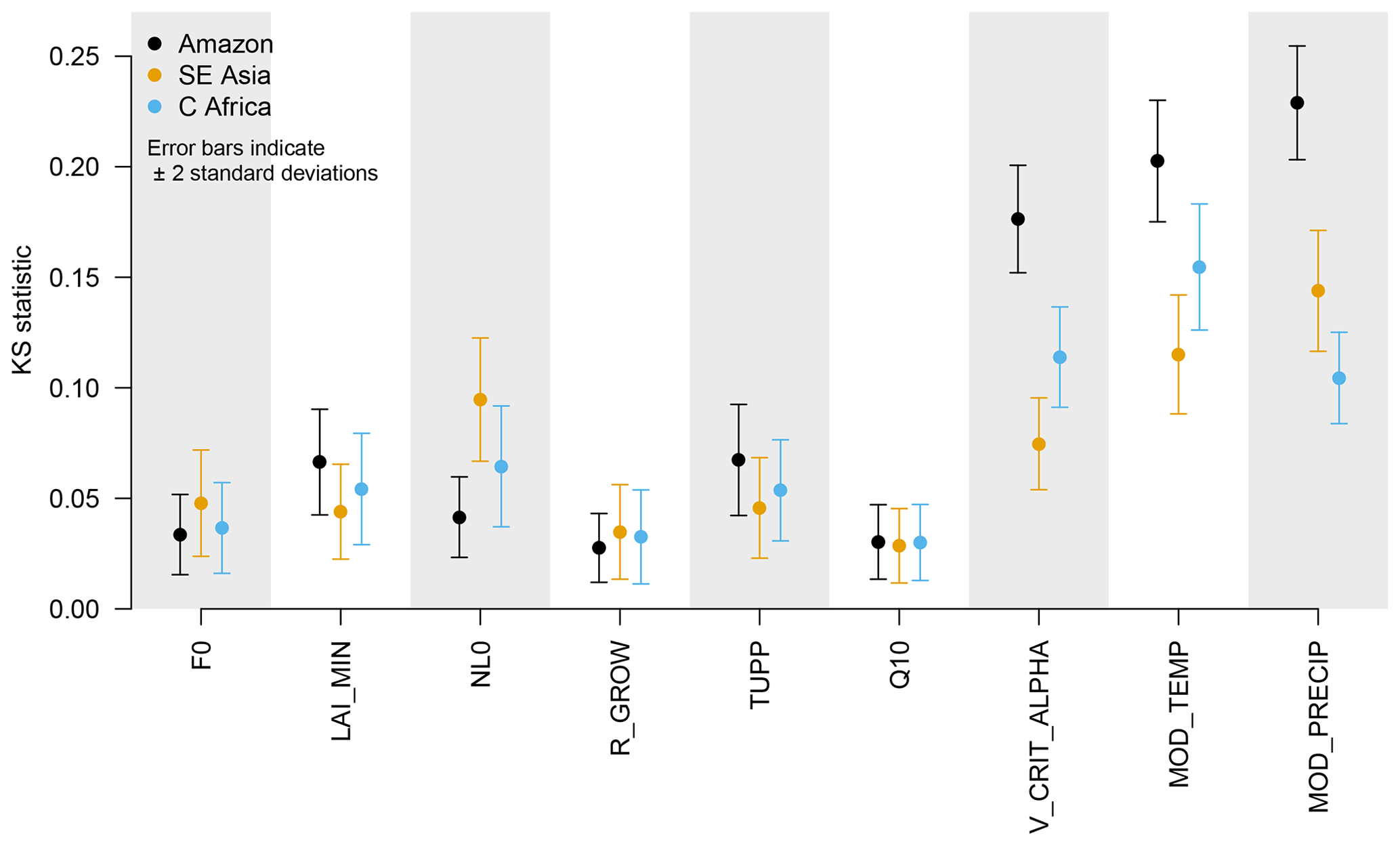
Figure 15Monte Carlo filtering estimate of the sensitivity of model output to inputs, using 5000 emulated members. Error bars represent ±2 standard deviations of uncertainty in the statistic, calculated by repeating the calculation 1000 times.

Download

We can check the strength of the relationship between the MCF sensitivity measures and the FAST99 sensitivity measures by plotting them together. We examine this relationship in the Supplement (Fig. S7).

4.5 Doing better than the default parameters

We can use the emulator to find locations in parameter space where there is a potential that the difference between the modelled and observed forest fractions could be smaller than at the default parameters. Figure 16 shows the density of parameter settings in each two-dimensional projection of the input space, where the emulator estimates the model performs better than at the default parameters, once bias correction has been applied. That is, the absolute difference between each estimated forest fraction and the observed values is smaller than the absolute difference of the mean estimate at the default parameters. Out of 100 000 samples from the uniform hypercube defined by the range of the experiment design, only 2451, or around 2.5 %, match this criterion and are plotted. This diagram might help guide further runs in the ensemble, choosing high-density regions to run new ensemble members. The convergence of NL0 and V_CRIT_ALPHA seems particularly focused and suggests that a lower value of V_CRIT_ALPHA might be a way to reduce error in the forest fraction. There is another, although less densely populated, region of high NL0 and V_CRIT_ALPHA that might fulfil the criteria of lower estimates of error for each forest. These regions would be good targets for supplementary runs of the climate model and for particularly careful emulator checking. A poorly performing emulator could guide a model developer into wasting model runs at locations which, in reality, did not produce forest fractions close to the observed values.

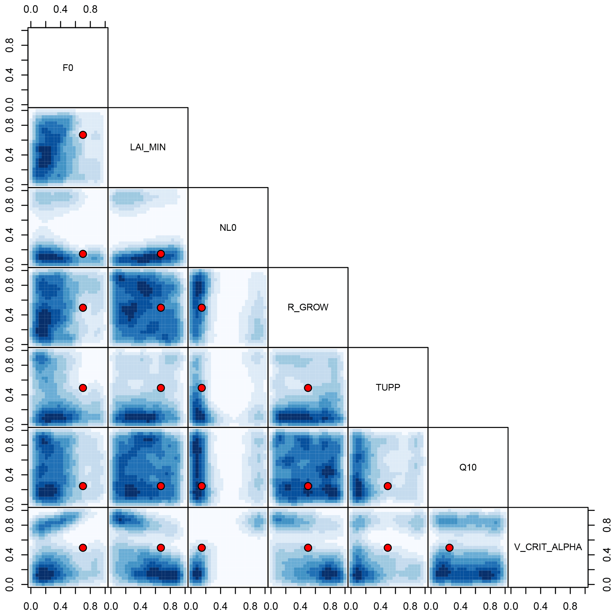
Figure 16Two-dimensional projections of the density of inputs where the corresponding bias-corrected emulated forests have a smaller error than the bias-corrected default parameters. These regions might be good targets for additional runs of the climate model. Default parameters are shown as a red point.

Download

4.6 Allowable climate at default parameters

We use history matching to find the set of regional mean climates that are most consistent with the observations for each tropical forest. To illustrate the best-case scenario, we set model discrepancy, its associated uncertainty and observational uncertainty artificially low (0, 0.01 and 0, respectively), so that implausibility is almost exclusively a product of the emulator uncertainty. We find the set of NROY temperature and precipitation values when the remaining input parameters are held at their default values. Figure 17 shows the density of NROY points in the climate space for each of the observed forest fractions. We see that the Amazon and central African forests might be well simulated in the model in a very wide range of cooler and wetter climates, with only the “hot, dry” corner showing zero density of potential inputs that produce similar forest fraction to observations. The southeast Asian forest fraction is matched by a swathe of inputs running diagonally through the centre of input space. Neither the hot, dry or cool, wet corners of input space produce forests that match the observations, though the warm, wet and cool, dry corners do.

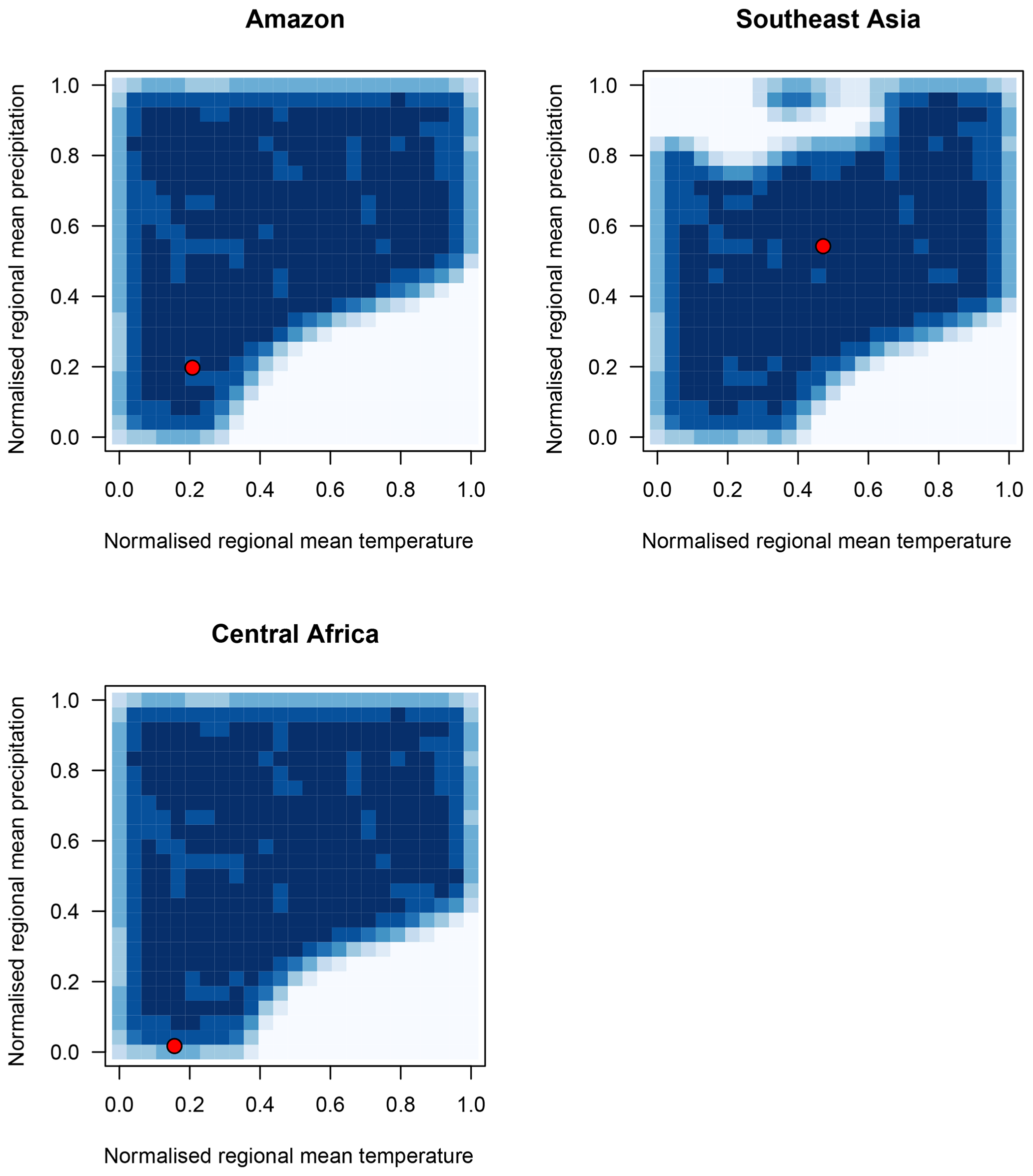
Figure 17Density of NROY emulated temperature and precipitation pairs for each observed tropical forest fraction, when input parameters are held at their default values. Observed climates for each forest are marked in red.

Download

5.1 Simulating the Amazon

We have shown that the simulation of the broadleaf tropical forest in FAMOUS is almost as sensitive to temperature and precipitation as to any land surface parameter perturbation in the ensemble. However, the calculated sensitivities are dependent on the chosen limits of the parameter perturbations themselves. The precise order and size of sensitivities might change given updated parameter ranges, but there is little doubt that the climate variables are a strong influence on broadleaf forest fraction. This version of FAMOUS when run with the default land surface input parameter settings would successfully simulate the Amazon rainforest to within tolerable limits if regional climate biases were substantially reduced. As such, there is no need to invoke a missing process in the land surface in order to explain the forest fraction discrepancy in the Amazon. We have strengthened the case made by M16 that the low Amazon forest fraction is not a result of poorly chosen parameters. There is a broad region of climate space where the effects of temperature and precipitation on forest fraction compensate for each other. This gives room for a number of possible sources of model discrepancy and by extension makes it unlikely that the default input parameters are optimal. There are indications from the emulator that a small region of parameter space exists where there is even smaller overall error in the simulation, offering a target for exploration using further runs of the model.

There is a feedback from the land surface to the atmosphere implicitly included in the emulated relationship. We cannot control this feedback directly with the emulator and thus work out the impact of this feedback on the forest fraction as it is present in the training data. This feedback would have to be taken into account if we were to simulate the correct climate independently of the land surface.

It is possible that were we to include a process seen to be missing from the Amazon (such as deeper rooting of trees allowing them to thrive in drier climates), our map of NROY input space would alter again. Given that there is a measure of uncertainty in observations and the emulator, as well as the possibility of further compensating errors, we cannot rule out a model discrepancy such as a deep rooting process. The fact that the other forests do slightly less well when their climates are bias-corrected points to a potential missing process in the model, compensated for by parameter perturbations. However, the impact of this missing process is likely much smaller than we might have estimated had we not taken the bias correction of the forest into account.

5.2 Uses for an augmented emulator

By building an emulator that includes temperature and precipitation – traditionally used as climate model outputs – we are able to separate the tuning of one component of the model (here the atmosphere) from another (the land surface). Perturbations to the atmospheric parameters, tested in a previous ensemble but not available to us except through an indicator parameter, are summarised as inputs through the climate of the model.

We have used the augmented emulator as a translational layer between components of the model. The augmented emulator allows us to ask what it would it mean for our choice of input parameters if the mean climate of the model in the Amazon region was correct. This means that we will have less chance of ruling out parts of parameter space that would lead to good simulations or keeping those parts that lead to implausible simulations. An augmented emulator as a translational layer might be built as part of a model development process, making it computationally cheaper and faster. Traditionally, the components of computationally expensive flagship climate models are built and tuned in isolation before being coupled together. The act of coupling model components can reveal model discrepancies or inadequacies. A model discrepancy in one model component can mean that a connected subcomponent requires retuning from its independently tuned state. There is a danger that this retuning leads to a model that reproduces historical data fairly well, but that makes errors in fundamental processes and therefore is less able to predict or extrapolate – for example, a climate model when projecting future changes under unprecedented greenhouse gas concentrations. Given the time and resources needed to run such complex models, these errors might persist much longer than necessary and have profound consequences for climate policy.

A translational layer would allow parameter choices to be made for a model when run in coupled mode, even when there was a significant bias in one of the components that would affect the other components. The translational layer would bias correct the output of a component of the model, allowing an exploration of the effects of input parameter changes on the subcomponent of the model, in the absence of significant errors. Using the augmented emulator could eliminate some of the steps in the tuning process, help the model developer identify potential sources of bias and quickly and cheaply calculate the impacts of fixing them. In doing so, it would aid model developers in identifying priorities for and allocating effort in future model development.

Our work here shows this process as an example. We have identified the importance of precipitation and temperature to the correct simulation of the Amazon forest and flag their accurate simulation in that region as a priority for the development of any climate model that hopes to simulate the forest well. We have identified regions of the space of these climate variables where the Amazon forest might thrive and related that back to regions of land surface parameter space that might be targeted in future runs of the model. We have achieved this in a previously run ensemble of the model, allowing computational resources to be directed towards new climate model runs that will provide more and better information about the model.

There are also potential computational efficiencies in our approach of decoupling the tuning of two components (here the atmosphere and the land surface) in the model. A good rule of thumb is that a design matrix for building an emulator should have O(10×p) training points, where p is the number of input parameters, in order to adequately sample parameter space to the extent it is possible to build a good emulator. With approximately 10 atmospheric and 7 land surface parameters, we would need O(170) runs. Here, we have summarised those 10 parameters as two outputs that have a material impact on the aspect of the land surface that we are interested in. Adding these two to the seven inputs, we need $O(\mathrm{10}\times (\mathrm{2}+\mathrm{7})=\mathrm{90})$ runs, well covered by our available ensemble of 100 runs.

We acknowledge, however, that in order to trace back information about the performance of the model in forest fraction to the original 10 oceanic and atmospheric parameters, we would need access to the original ensemble. We have used temperature and precipitation to reduce the dimension of the parameter space, but there is no guarantee that the relationship between the original parameters and the local climate is unique. There may be multiple combinations of the 10 parameters that lead to the temperature and precipitation values seen, which would mean that we would require a large ensemble to estimate the relationships well. Alternatively, there may be an even more efficient dimension reduction for forest fraction, meaning we would need even fewer model runs to summarise the relationship.

5.3 Limitations

In theory, the augmented emulator could be used to bias correct differently sized regions, down to the size of an individual grid box for a particular variable. This might be useful for correcting, for example, known biases in elevation or seasonal climate. The principle of repeating the common parameter settings in the design matrix, and including model outputs as inputs, would work in exactly the same way but with a larger number of repeated rows. In the case of using an augmented emulator on a per-grid-box basis, we might expect the relationship between inputs that we are bias correcting (e.g. temperature, precipitation) and the output of interest (e.g. forest fraction) to be less clear, as at small scales there are potentially many other inputs that might influence the output. An emulator for an individual grid box might therefore be less accurate. However, with enough data points, or examples (and there would be many), we might expect to be able to recover any important relationships.

The computational resources needed to fit a Gaussian process emulator when the number of outputs estimated simultaneously becomes even moderately large limits the use of our technique. The design input parameter matrix used for training the emulator grows to n×d rows, where n is the number of ensemble members in the original training set, and d is the number of separate output instances to be considered. In our example, d is 3, and so we only have $\mathrm{100}\times \mathrm{3}=\mathrm{300}$ in the new training set. Given an initial ensemble of a few hundred, this could easily result in a training set with hundreds of thousands or even millions of rows. Gaussian process emulators are currently limited to using training data with perhaps a few hundred rows as current software packages must invert an n×n matrix, a potentially very computationally expensive process (Hensman et al., 2013, see, e.g.). At the time of writing, this limitation would preclude using our specific technique for correcting biases on a per-grid-box basis. To make use of the translational layer for large data sets, we would need new Gaussian process technology or specific strategies to deal with large data sets. These strategies might involve kernel-based methods, keeping the scope of training data local to limit the size of any inverted matrices. Alternatively, they might involve building emulators using only a strategically sampled selection of the outputs. Recent advances in using Gaussian processes for larger data sets can be found in Hensman et al. (2013, 2015); Wilson et al. (2015); Wilson and Nickisch (2015). Our current strategy is to reduce the dimension of the output of the climate model by taking the regional mean of the output of the climate model (temperature and precipitation). More advanced dimension reduction techniques might offer great potential.

Given that we overcome such technical barriers, we see no reason that such a layer not be built that is used to (for example) correct the climate seen by individual land surface grid boxes rather than (as here) individual aggregated forests. The process of rejecting poor parameter sets might be aided by having a comparison against each grid box in an entire global observed surface, rather than aggregated forests. Alternatively, we might allow parameters to vary on a grid-box-by-grid-box basis, effectively forming a map of NROY parameters.

If trained on an ensemble of model runs which included all major uncertainties important for future forests, an augmented emulator could be used directly to estimate the impacts and related uncertainty of climate change on forest fraction in the model, even in the presence of a significant bias in a model subcomponent. After estimating the relationship between the uncertain parameters, climate and the forest fraction, we could calculate the forest fraction at any climate, including those that might be found in the future. This ensemble of climate model runs would project the future forests under a number of atmospheric CO₂ concentrations and parameter combinations. It would be necessary that the training data included any climates that might be seen under the climate change scenario to be studied, as the emulator has much larger uncertainties if asked to extrapolate beyond the limits of the training data. The trajectory of vegetation states through time would also be an important element of the ensemble, as the vegetation state is path dependent. However, there would be great potential to save a large number of runs, as not every parameter perturbation would have to be run with every projection scenario. Such a set of runs would serve as a framework upon which a great many post hoc analyses could be done with the emulator. Once the set of runs was complete, they would effectively serve as the definitive version of the model – any new information that needed to be extracted from the model could in theory be found using the emulator. Not only might we be able to identify and correct important climate biases and their impact on the forest but also to update our estimates of forest change as we learn more about the uncertainty ranges of the uncertain parameters and forcing trajectory.