We develop and implement a computationally efficient surrogate of the MEGAN3.0 canopy model (https://bai.ess.uci.edu/megan, last access: 4 September 2019), an update from previous versions of MEGAN (Guenther et al., 2006, 2012). This canopy model calculates leaf temperature and leaf-level PAR for a five-layer plant canopy for both sunlit and shaded leaves, whereby each canopy layer represents a fraction of the total plant canopy. The model is originally based largely on Goudriaan and Laar (1994) and a brief description follows; for more information see Guenther et al. (1999, 2006, 2012).

In the MEGAN3 canopy model the fraction of sunlit leaves in the canopy decreases exponentially as a function of the local solar elevation angle, canopy leaf area index (LAI), a clustering coefficient that accounts for leaf geometries, and a canopy transparency coefficient representing the fraction of the canopy that does not intercept incident radiation. The leaf temperature is calculated from a system of energy balance equations based on Goudriaan and Laar (1994) and Leuning et al. (1995), with a maximum absolute difference between the air temperature and leaf temperature of 10 ^∘C. Leaf-level PAR is computed as a function of incoming radiation incident to the canopy top, the sunlit fraction of leaves, LAI, and a suite of geometric and radiative lookup table characteristics, predominantly based on Goudriaan and Laar (1994), Leuning et al. (1995), and Spitters (1986). The full MEGAN3 canopy model takes as input time (day and hour), geographical location (latitude and longitude), air temperature, incident radiation on the top of the canopy, wind speed, humidity, air pressure, LAI, and a set of canopy characteristics (canopy biomass distribution, clustering coefficients, etc.) in the form of a lookup table that varies by six vegetation types. The six vegetation types are needleleaf trees, tropical forest trees, temperate broadleaf trees, shrubs, herbaceous plants, and crops. It is important to note that differing canopy model choice and parameter selection can result in substantial changes to the ultimate estimates of biosphere–atmosphere exchange (Keenan et al., 2011). The MEGAN3 canopy model has been specifically developed for use in simulating biogenic emissions and has been extensively applied in related studies (e.g., Chen et al., 2018; Geron et al., 2016; Guenther et al., 2006). Additionally, the MEGAN framework has been widely adopted across a variety of regional and global models (e.g., GEOS-Chem, WRF-CHEM, and CESM). Thus, the MEGAN3 canopy model is a good candidate for surrogate model development because it enables a direct implementation of improved process-based canopy physics into a variety of 3D models without the need for substantial model architecture development.

To begin the surrogate model development, we first use a variable selection approach to evaluate and rank which of the suite of model input variables are most important for the simulation of both leaf-level PAR and temperature. To do this, we use a machine-learning regression method for model simplification and parameterization, specifically LASSO (least absolute shrinkage and selection operator; Hastie et al., 2001). As applied here, LASSO is a regression method that calculates linear coefficients through a modified least squares cost function, with the addition of a penalized L1 norm (the sum of the absolute value of the coefficients). While LASSO was originally developed as a complete regression method, we follow the recommendations of Hastie et al. (2001) and use LASSO only for variable importance ranking and dimensionality reduction of the input variable space to the model.

We apply the linear LASSO method for rankings across a full year of 3-hourly simulated canopy physics from the MEGAN3 canopy model at the global scale for the year 2012. Input meteorology is from MERRA-2 assimilated meteorological fields at $\mathrm{2}{}^{\circ }\times \mathrm{2.5}{}^{\circ }$ horizontal resolution (Gelaro et al., 2017) and the vegetation distribution from the Olson et al. (2001) land maps. LAI is derived from the MODIS TERRA MOD15A2 product (Myneni et al., 2002, 2007) regridded to $\mathrm{2}{}^{\circ }\times \mathrm{2.5}{}^{\circ }$ horizontal resolution and a monthly timescale. These input data are identical to those used in the GEOS-Chem chemical transport model (CTM), described below for direct comparison with prior work and ease of implementation into that CTM. The spatial distribution of vegetation and LAI is summarized in Figs. 1 and 2, respectively. In general, forested land classes have the highest LAI values and are spread throughout the tropics and the northern latitudes. Crops, grasses, and shrubs are located predominantly in transitionary landscapes and near regions of larger population (e.g., India, central North America, etc.), and they tend to have lower LAI values.

Figure 1The percent of each $\mathrm{2}{}^{\circ }\times \mathrm{2.5}{}^{\circ }$ grid box occupied by each vegetation class used in this work. Panel (a) is forested vegetation, and panel (b) is crops, grasses, and shrubland.

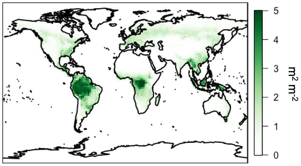
Figure 2Annual average LAI from MODIS for the year 2012.

The LASSO importance rankings are remarkably consistent for both sunlit and shaded leaves and for all vertical levels of the canopy. For each quantity, the two highest ranked variables are consistent at each layer throughout the canopy and have substantially larger importance to the final result than any additional variable. For brevity we discuss only those first two variables here. The two most important variables for the calculation of leaf temperature are air temperature and wind speed. Air temperature dominates in importance for the calculation of leaf temperature, with a larger coefficient emerging at a higher L1 norm penalty weighting. Other variables that are physically important in nature (e.g., solar radiation) do not appear important in the LASSO rankings due in part to how they covary with air temperature and how the rankings are derived separately for sunlit and shaded leaves. For the calculation of leaf PAR we find that the two most important variables are PAR out of the lowermost atmospheric grid box (incident on the canopy) and the local vegetation LAI. We use these selected variables to develop a simplified parameterization for leaf temperature and PAR.

We model leaf temperature for a given canopy level, i (T_i,leaf, K), as linear with 2 m air temperature (T_air, K):

where A_i and B_i are fitted parameters per canopy level (i). This ignores the addition of the second most important variable, wind speed. However, the addition of wind speed to the regression only improves the performance of the model by less than 1 % in total bias and R²; thus, for simplicity, we neglect this variable.

For the calculation of leaf-level PAR at a given canopy level (PAR_i,leaf, $\mathrm{\mu }\mathrm{mol}{\mathrm{m}}^{-\mathrm{2}}{\mathrm{s}}^{-\mathrm{1}}$), we use an exponential Beer's law analog, including the influence of leaf area index (LAI) and the PAR incident to the top of the canopy (PAR_toc, W m⁻²):

where C_i and D_i are fitted parameters per canopy level (i). This exponential functional form is chosen due to the observed and simulated relationships between LAI and canopy light interception (Engel et al., 1987; Goudriaan and Monteith, 1990) following a similar functional form.

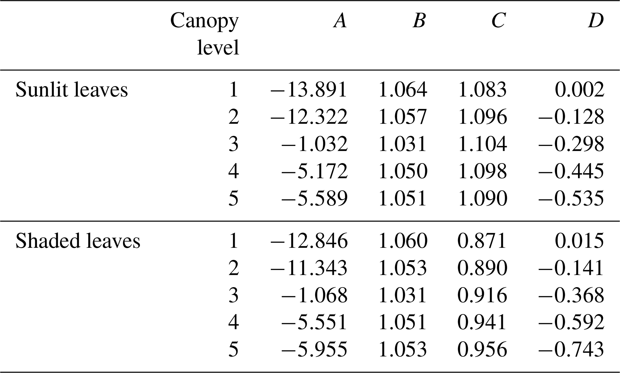
We fit Eqs. (1) and (2) for all layers of the canopy and for sunlit and shaded leaves, resulting in 20 total free parameters necessary to model the entire plant canopy across the globe. In this regression method, we ignore the role of differing vegetation classes and apply the regression agnostic to vegetation type. This is done to keep the total necessary number of free parameters low (20 versus 120) and because this more parsimonious model performs quite well (see Sect. 3.1) without the need for additional vegetation-type-specific coefficients. The resulting surrogate model coefficients are summarized in Table 1.

Table 1Regression coefficients for the canopy surrogate model. Canopy level 1 represents the top of the canopy.

Download Print Version | Download XLSX

The final quantity necessary for the canopy model is the fraction of sunlit and shaded leaves. Here, that fraction in each layer of the plant canopy is calculated directly following the MEGAN3 code (see Guenther et al., 2006, 2012), without any model simplification. The sunlit fraction is calculated as follows:

where β is the solar angle above the horizon, K_b is the extinction coefficient for black leaves, C₁ is the canopy-clustering coefficient, C₂ is the canopy transparency, and f is the fraction of biomass in the canopy light travels through to reach a given leaf (the vector [0.05, 0.23, 0.5, 0.77, 0.95]). Consistent with the MEGAN3 parent canopy model, we assume a Gaussian distribution of biomass in the canopy, centered in the middle canopy layer, a canopy transparency of 0.2, and a leaf-clustering coefficient of 0.9.

From this relatively simple three-function parameterization (leaf temperature, leaf PAR, and sunlit leaf fraction), we are able to implement more physically realistic parameterizations for biosphere–atmosphere interactions in atmospheric chemical transport models.

3.1 Surrogate model performance

Here, we evaluate the surrogate model performance for all vegetation globally.

3.1.1 Temperature

The surrogate-model-simulated annual canopy average leaf temperature distribution and performance for 2012 are summarized in Figs. 3 and 4. In Fig. 3, the average for each canopy layer is calculated as a sum of the sunlit and shaded leaves, weighted by the sunlit fraction of that layer. In turn, the canopy average is calculated as the weighted sum of the layer averages, weighted by the fraction of the canopy biomass in each layer. The annual average temperature is shown in Fig. 3a, where it largely follows a latitudinal gradient. The warmest temperatures are ∼310 K in the tropics, and the coldest average leaf temperatures are ∼280 K in the northern high-latitude boreal regions. The surrogate model is linear with the 2 m “near-surface” air temperature and therefore follows that spatial distribution directly.

The surrogate model for leaf temperature performs well, with the annual average spatial R² and mean bias relative to the full model shown in Fig. 3b and c, respectively. Across all regions, the R² is very high, indicating that a linear relationship between 2 m air temperature and canopy average temperature is a good approximation for capturing the variability of the full MEGAN3 canopy model. The temperature R² drops below 0.90 only in coastal regions and grid boxes that contain very little vegetation, representing less than 5 % of all vegetated areas. The temperature surrogate bias is also generally quite low, as shown in Fig. 3c. The majority of regions have an absolute mean bias of less than 1 K, and more than 90 % of the annual average mean biases are less than 2 K. The surrogate model generally computes temperatures that are biased cool over highly vegetated tropical and subtropical regions, and it slightly overestimates temperature over northern boreal forests (by ∼0.1 K). The most substantial overestimations occur in or near the hot and arid regions of the globe and always in regions where there is little vegetative cover at all. On a relative scale these biases are quite small; all are less than 1 % of the total magnitude. The model development process described in Sect. 3 removed the vegetation type discrimination in the parent MEGAN3 canopy model. This leads to some spatial coherence in the global bias patterns, whereby regions dominated by coniferous forests, grasses, and shrubs (e.g., boreal Northern Hemisphere and the western United States) tend to be slightly biased warm, and the other vegetation types are biased slightly cool.

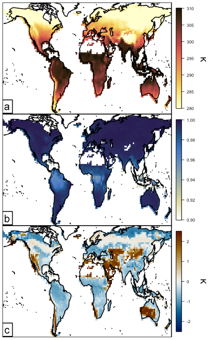
Figure 3Surrogate model performance for the annual canopy average leaf temperature in 2012. Panels are as follows: (a) annual average surrogate model leaf-level temperature (Kelvin), (b) R² between the surrogate and the full model leaf-level temperature, and (c) annual average leaf-level temperature bias (surrogate–full model, K).

The vertical profile of annual average leaf temperature is shown in Fig. 4a. The broad shape of the canopy profile is consistent across vegetation types and the globe. The upper canopy layers are cooler than the lower canopy layers, as an insulating effect from air temperature occurs within the canopy. The higher-order variability (e.g., small differences between adjacent layers at the top and bottom of the canopy) stems from the more detailed representation of canopy energy balance in the full MEGAN3 model, which includes the influence of terms like PAR, relative humidity, LAI, and wind speed. However, this higher-order variability is quite consistent, allowing it to be reproduced in the simplified surrogate model.

Similar to the spatial performance, the overall surrogate model performs well throughout the canopy. The surrogate model temperature R² is shown in Fig. 4b. The values are all near 1.0, with the lowest value of 0.97 in the middle of the canopy, where the transition from cooler to warmer leaves is slightly more difficult for the surrogate model to capture. As demonstrated in Fig. 4c, the bias throughout the canopy is low as well. On a global annual average, the surrogate model is biased cool but only slightly (on both a relative and absolute scale). The highest-magnitude bias is at the top canopy layer at −0.04 K.

Figure 4Surrogate model performance for the annual average vertical canopy temperature profile in 2012. Panel (a) shows the vertical average surrogate model leaf-level temperature (Kelvin). Panel (b) shows the surrogate model R² against the full model. Panel (c) shows the leaf-level temperature bias (K) of the surrogate model compared to the full model.

Download

3.1.2 Photosynthetically active radiation

The annual canopy average leaf-level PAR for 2012 is shown spatially in Fig. 5a. In Fig. 5, canopy temperature averages are calculated using the same method as for canopy temperature. Annual average PAR varies from ∼200 $\mathrm{\mu }\mathrm{mol}{\mathrm{m}}^{-\mathrm{2}}{\mathrm{s}}^{-\mathrm{1}}$ to greater than 600 $\mathrm{\mu }\mathrm{mol}{\mathrm{m}}^{-\mathrm{2}}{\mathrm{s}}^{-\mathrm{1}}$. This spatial variability is a function of both PAR incident on the top of the canopy (largely related to cloud cover and solar angle) and the canopy LAI. Leaf-level PAR in the surrogate model varies linearly with incident PAR and decreases exponentially with LAI. Additionally, the reduction under high LAI is exacerbated due to a higher fraction of shaded leaves in high-LAI canopies, which have substantially lower average PAR. The highest leaf-level PAR values are generally located in arid regions, where LAI and the number of cloudy days are quite low. The lowest values are located in the equatorial tropical rainforests and the northern boreal forests. The low leaf-level PAR values in the rainforest are coincident with the highest LAI values globally, leading to very strong shading effects below the first canopy layer. The northern boreal forests have low leaf-level PAR, in part due to relatively high LAI but also due to reduced incoming PAR in the winter months when the solar angle is low.

The annual average performance of the surrogate leaf-level PAR relative to the full model is shown in Fig. 5b and c. The temporal R² over a full year in Fig. 5b is generally quite high, indicating that the surrogate formulation captures the majority of the temporal variability inherent in the full model. The R² values range from 0.92 to 1.0. The highest R² values are in regions with low LAI, where the effects of shading and other canopy physical processes are greatly reduced. The worst model R² performance is over two characteristic regions: higher elevations with low vegetation densities (i.e., global deserts in Central Asia and South America) and those with the highest LAI. Both regions represent extreme scenarios for canopy radiative physics. The higher-elevation regions with low vegetation densities have very little leaf shading at all throughout the year, and thus the canopy physics represented with a simple exponential decay are no longer as relevant. In the high-LAI regions, the elevated importance of shading and resulting complexity in the PAR calculation are more challenging for the simplified representation of the surrogate model. However, this poor performance still has a quite high R², with the lowest value of 0.92. The annual average model biases are generally within ±40 $\mathrm{\mu }\mathrm{mol}{\mathrm{m}}^{-\mathrm{2}}{\mathrm{s}}^{-\mathrm{1}}$, with a few more extreme values reaching ±200 $\mathrm{\mu }\mathrm{mol}{\mathrm{m}}^{-\mathrm{2}}{\mathrm{s}}^{-\mathrm{1}}$. The surrogate model is broadly biased high over regions with lower LAI and slightly low over regions with high LAI. In a relative sense, these changes are nearly all within 10 %–15 %, with a maximum normalized mean bias of 0.4.

Figure 5Surrogate model performance for the annual canopy average leaf PAR in 2012. Panels are as follows: (a) annual average surrogate model leaf-level PAR ($\mathrm{\mu }\mathrm{mol}{\mathrm{m}}^{-\mathrm{2}}{\mathrm{s}}^{-\mathrm{1}}$), (b) R² between the leaf-level PAR simulated using the surrogate and the full model, and (c) annual average leaf-level PAR bias (surrogate–full model, $\mathrm{\mu }\mathrm{mol}{\mathrm{m}}^{-\mathrm{2}}{\mathrm{s}}^{-\mathrm{1}}$).

The average vertical distribution of leaf-level PAR throughout the canopy and the associated surrogate model performance are shown in Fig. 6. To explore the additional dependence on LAI, the quantities shown are separated into three LAI ranges. These are as follows: a low range with LAI less than 0.5, a midrange with LAI between 0.5 and 5, and a high-LAI range containing canopies with a total LAI greater than 5. The low LAI range represents ∼40 % of all vegetation throughout the year, the middle range represents nearly 60 %, and the high-LAI range contains only a small fraction of all vegetation (∼1 %).

The average distribution of PAR across canopy levels is shown in Fig. 6a. As LAI increases, there is a substantial reduction in leaf-level PAR deeper into the vegetated canopy. This is particularly obvious with the high-LAI range, consistent with substantial shading and light interception above the bottom of densely vegetated canopies. On the other hand, the variability throughout the low-LAI canopies is quite small. This LAI dependence explains in part the relatively low canopy average leaf-level PAR throughout the tropical forests in Fig. 5a. The variability in the PAR at the top canopy layer (canopy level 1 in Fig. 6a) stems from two major sources. The first is simply the spatial distribution of these LAI ranges in relationship to the annual average incident PAR to the canopy top. Very high LAI values occur primarily over the tropics, where sunlight is consistently high throughout the year and the seasonal effects of changing solar angles is small. The opposite is true for many of the regions with smaller LAI values, which are distributed more evenly across the globe. A second-order effect in the MEGAN3 canopy model is that of in-layer attenuation of light and shading throughout the canopy, whereby leaves in a given layer may intercept light and shade leaves lower within that same layer. This has the effect of reducing the layer average leaf-level PAR as a function of leaf geometries and LAI, and it explains why the highest canopy layer average leaf-level PAR is not the same as the average PAR incident on the top of the canopy.

Figure 6b and c summarize the statistical performance of the surrogate model vertically through the canopy in terms of the R² and the mean bias, respectively. Overall, the surrogate model reproduces the PAR variability compared to the full parent model well. For both the low and middle LAI ranges (LAI less than 5), all R² values are greater than ∼0.9. The only substantially lower R² values are from the lower canopy in high-LAI regions, where PAR is generally quite small (see Fig. 6a). The surrogate model struggles somewhat to capture this lower canopy variability, due in large part to the increased complexity of resolving canopy shading and radiative physics in high-LAI canopies. However, the ultimate influence on the total canopy-scale bias is generally low.

The vertical distribution of that bias is shown in Fig. 6c. Broadly, the absolute PAR bias is low (less than 5 % on a relative scale) and decreases throughout the canopy. All biases are positive except for the top canopy layer for high-LAI-range canopies; this poor fit is likely related to the limited representation of high-LAI regions in the full dataset (only ∼1 % of all vegetated area) and is not present if a lower cutoff for high LAI ranges is used (e.g., LAI >3). The decreasing magnitude throughout the canopy is largely related to the decreasing overall leaf-level PAR (see Fig. 6a). It important to note that the bias terms are all sensitive to the choice of LAI bin ranges, and the variability in bias at each level can be quite large (e.g., above 50 $\mathrm{\mu }\mathrm{mol}{\mathrm{m}}^{-\mathrm{2}}{\mathrm{s}}^{-\mathrm{1}}$ in the top canopy layer). For both the high and middle LAI ranges, the absolute magnitude of the PAR bias decreases throughout the canopy, and the bias remains relatively constant for low-LAI-range vegetation. On a relative scale, these biases are all quite small, with a normalized mean bias usually less than 5 %. The exception to this is the lowest layer of the high-LAI-range canopies. In this low canopy layer the magnitude of the bias is quite low, as is the total magnitude of leaf-level PAR; the resulting difference between small numbers leads to a relatively large normalized mean bias of ∼0.3.

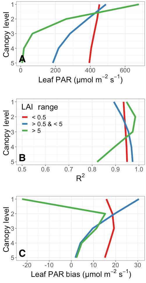
Figure 6Surrogate model performance for the annual average vertical canopy PAR profile in 2012 as a function of LAI. Panel (a) shows the vertical average surrogate model leaf-level PAR ($\mathrm{\mu }\mathrm{mol}{\mathrm{m}}^{-\mathrm{2}}{\mathrm{s}}^{-\mathrm{1}}$) for low-LAI (red), midrange LAI (blue), and high-LAI canopies. Panel (b) shows the surrogate model R² against the full model. Panel (c) shows the leaf-level PAR bias ($\mathrm{\mu }\mathrm{mol}{\mathrm{m}}^{-\mathrm{2}}{\mathrm{s}}^{-\mathrm{1}}$) of the surrogate model compared to the full model. Level 1 is the top of the canopy.

Download

An essential function of canopy models used in CTMs is to calculate the amount of light that falls on already light-saturated leaf surfaces. This regulates the effect of a change in PAR incident on the canopy on various biological and physical processes (e.g., biogenic emissions). We estimate the fraction of leaves that are light-saturated using the γ_PAR formulation from the MEGAN algorithm (Guenther et al., 2006, 2012). This variable aims to capture the amount of light saturation on a given leaf and ranges from 0 to 1, with higher values corresponding to more saturated leaves. To explore light saturation, we examine cases in which the γ_PAR value is greater than 0.9. A scatterplot of the annual average fraction of leaves that are light-saturated (γ_PAR≥0.9) per model grid box for both the full model and the surrogate model throughout the canopy is shown in Fig. 7. The surrogate model reproduces the full model fraction of light-saturated leaves well, generally to within ∼5 %, with a median bias of −2 %.

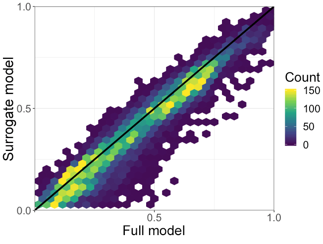
Figure 7The annual grid box average fraction of light-saturated leaves as simulated by the full and surrogate models throughout the canopy for the year 2012. The color bar represents the number of observations in a given hex. The 1:1 line is shown in black.

Download

Ultimately, this assessment demonstrates that the surrogate model reproduces the parent MEGAN3 canopy model well for both leaf temperature and leaf-level PAR. The exponential relationship between leaf-level PAR and canopy incident PAR and the linear relationship between leaf temperature and near-surface air temperature capture the majority of the information inherent in the parent model. Some higher-order variability in the absolute magnitude of the variables is missing from this surrogate model; however, the biases are generally all within ∼10 %.

We evaluate the impact of the canopy model parameterization on atmospheric composition using the GEOS-Chem v12.3.0 chemical transport model (http://www.geos-chem.org, last access: 30 May 2020, https://doi.org/10.5281/zenodo.2620535, The International GEOS-Chem User Community, 2019). GEOS-Chem is a computational model for simulating atmospheric chemistry, including a detailed HO_x–NO_x–BrO_x tropospheric chemical mechanism (Bey et al., 2001; Mao et al., 2013; Travis et al., 2016). We drive GEOS-Chem with MERRA-2 meteorology at $\mathrm{2}{}^{\circ }\times \mathrm{2.5}{}^{\circ }$ spatial resolution with 47 vertical layers (Gelaro et al., 2017). The time steps for convection and chemistry are 10 and 20 min, respectively. Identically to the canopy model input data, we use LAI values from the MODIS Terra MOD15A2 product (Myneni et al., 2002, 2007) and plant functional types (PFTs) from the Olson et al. (2001) dataset. Fire emissions are from the Global Fire Emissions Database v4 (GFED4; Giglio et al., 2013), and global anthropogenic emissions are from the Community Emissions Data System inventory (CEDS; Hoesly et al., 2018). Regional emissions over the United States, Africa, and Asia are from the NEI 2011 (Travis et al., 2016), DICE-Africa (Marais and Wiedinmyer, 2016), and MIX (Li et al., 2017) emissions inventories, respectively. Soil NO_x emissions are calculated following Hudman et al. (2012). Simulations are shown for the years 2012 and 2013, with the first year discarded for spin-up when considering gas-phase chemical impacts.

4.1 MEGAN emissions

The biogenic emissions scheme in GEOS-Chem v12.3.0, MEGAN2.1, is based on Guenther et al. (2006, 2012) and Millet et al. (2010). The emissions of a given compound are calculated from base canopy-level emission factors multiplied by “activity factors” representing standard processes that govern biogenic emissions (temperature, PAR, light dependence, etc.) and “stress factors” modeling the effect of vegetative stress (heat, drought, etc.) on biogenic emissions. Each of these activity and stress factors vary with the environmental state. The base emission factor itself varies with vegetation type, and these activity factors respond to leaf temperature, leaf-level PAR, leaf age, leaf area index, soil moisture, and atmospheric CO₂ concentrations. The base emission factors used in this work are consistent with those used in GEOS-Chem v12.3.0; an example for isoprene is shown in Fig. 8. The emission factors are highest in forested regions and lowest over areas with little vegetation (e.g., deserts). These emission factors are regridded from the original resolution of $\mathrm{0.25}{}^{\circ }\times \mathrm{0.3125}{}^{\circ }$ to match the GEOS-Chem resolution of $\mathrm{2}{}^{\circ }\times \mathrm{2.5}{}^{\circ }$.

Figure 8Base isoprene emission factors used in this work.

As GEOS-Chem v12.3.0 has no representation of plant canopy physics, the LAI, temperature, and PAR activity factors are all reparameterized following Guenther et al. (2006) in the standard model. In this parameterization, leaf temperature is assumed to equal air temperature in the calculation of the temperature activity factor. The LAI and PAR activity factors are calculated in an approach known as the parameterized canopy environment emission activity (PCEEA) approach that does not include any description of the vertical distribution of vegetation and only includes responses to the LAI, PAR incident to the top of the canopy, and the solar zenith angle.

We modify the MEGAN implementation in GEOS-Chem to allow for the representation of canopy physics described in Sect. 3. In order to properly scale all emission factors to the plant canopy using a canopy model, a normalization factor must be applied at a set of standard environmental and ecological conditions (Guenther et al., 2006, 2012). This normalization factor varies depending on the choice of those standard conditions and the canopy model used. In MEGAN2.1 these standard conditions are LAI of 5, current air temperature of 303 K, current incident PAR at the canopy top of 1500 $\mathrm{\mu }\mathrm{mol}{\mathrm{m}}^{-\mathrm{2}}{\mathrm{s}}^{-\mathrm{1}}$, and a 10 %∕80 %∕10 % split of growing, mature, and senescent leaves (Guenther et al., 2012; Kaiser et al., 2018). We calculate other necessary standard conditions, specifically the 24 h average air temperature and PAR, from the meteorological fields conditional on locations that meet the previously described standard conditions. In situations in which all of the previous instantaneous standard conditions (e.g., current temperature 303 K, current PAR 1500 $\mathrm{\mu }\mathrm{mol}{\mathrm{m}}^{-\mathrm{2}}{\mathrm{s}}^{-\mathrm{1}}$, and LAI 5) are jointly met to within ±10 %, we calculate the 24 h average prior meteorological conditions from the global reanalysis fields and use the mean of those calculations as the standard 24 h average conditions. The resulting standard conditions for 24 h average temperature and 24 h average PAR are 298.5 K and 740 $\mathrm{\mu }\mathrm{mol}{\mathrm{m}}^{-\mathrm{2}}{\mathrm{s}}^{-\mathrm{1}}$, respectively. These standard conditions result in a normalization factor of 0.21 using the surrogate canopy model developed in this work. The value of 0.21 is lower than those used in implementations of previous MEGAN model versions in other models such as CLM (0.3) and WRF-Chem (0.57) (Guenther et al., 2012). It is important to note that the normalization factor approximately scales with the square of the current temperature conditions and linearly with the current PAR conditions. For the 24 h average conditions, the scaling is reduced to approximately linear for temperature and as a square root for PAR. Given this, small deviations from these standard conditions (e.g., those that could arise from different 24 h averaging methodology) can lead to substantial changes in the normalization factor. Additionally, consistent with previous work these standard conditional calculations are likely variable across model meteorological configurations and should be recalculated on a model-specific basis (Guenther et al., 2012). Since this normalization factor is applied consistently to all emissions globally at all times, it linearly modulates all biogenic emissions. As such, the total emissions calculated by the MEGAN2.1 emissions framework are highly sensitive to the parameter choices made in this normalization processes.

In GEOS-Chem v12.3.0 we update the activity factors associated with PAR, LAI, and temperature as well as the normalization to take advantage of our new canopy surrogate model. This enables a full implementation of the most recent MEGAN3 emission activity algorithm in the GEOS-Chem model. In the PCEEA implementation of MEGAN in the base version of GEOS-Chem, activity factors are calculated separately for PAR (γ_P), LAI (γ_LAI), and temperature (γ_T) and then multiplied together following Guenther et al. (2006):

$$\begin{array}{}\text{(5)}& {\displaystyle }{\mathit{\gamma }}_{\mathrm{PCEEA}}={\mathit{\gamma }}_{\mathrm{LAI}}{\mathit{\gamma }}_T{\mathit{\gamma }}_{\mathrm{P}}.\end{array}$$

Following MEGAN3, we implement PAR and temperature activity factors that are calculated jointly per canopy level and summed together weighted by the vertical canopy biomass distribution. In this work, as in previous non-PCEEA versions of the MEGAN framework (Guenther et al., 2006, 2012), the effect of LAI is calculated through direct multiplication of the emission factor by LAI as opposed to an activity factor formulation, along with a canopy normalization factor (C_CE).

$$\begin{array}{}\text{(6)}& {\displaystyle }& {\displaystyle }{\mathit{\gamma }}_{\mathrm{Canopy}}=C_{\mathrm{CE}}\mathrm{LAI}{\mathit{\gamma }}_{\mathrm{TP}}\text{(7)}& {\displaystyle }& {\displaystyle }{\mathit{\gamma }}_{\mathrm{TP}}=\sum _{l=\mathrm{1}}^{\mathrm{5}}{w}_{\mathrm{l}}{\mathit{\gamma }}_{\mathrm{P}}{\mathit{\gamma }}_T\end{array}$$

These activity factors for PAR, LAI, and temperature are the same as those in Guenther et al. (2012) as averages throughout the canopy weighted by the biomass fraction within a given canopy layer (w_l). There is an additional canopy depth emission activity response applied to the light-dependent activity factors, which is intended to model the variability of emissions throughout the canopy (e.g., Harley et al., 1996). This canopy depth activity factor is a multiplicative factor that varies linearly as a function of LAI and canopy depth, with a value between 0 and 1.3. For clarity, we refer to the MEGAN emissions implementation in GEOS-Chem using the γ_PCEEA activity factors as “MEGAN_PCEEA” and those using the γ_Canopy activity factors as “MEGAN_Canopy”. While γ_T in the MEGAN_PCEEA approach follows a similar functional form to that in MEGAN_Canopy, the lack of vertical canopy structure in the MEGAN_PCEEA configuration leads to a very different treatment of the joint effects of temperature, PAR, and LAI on emissions. Specifically, the MEGAN_PCEEA approach aims to approximate the joint effects of shading and temperature change within a canopy, whereas MEGAN_Canopy aims to directly simulate those processes. We use the canopy physics surrogate model described in Sect. 3 to calculate the leaf temperature and PAR in the MEGAN_Canopy implementation.

Though stress factors in the MEGAN framework allow for the additional capability to evaluate the impact of vegetative stress processes on emissions (e.g. Geron et al., 2016), we do not enable those processes in this study. The other activity factors (leaf age, soil moisture, and CO₂ inhibition) are the same in both MEGAN_Canopy and MEGAN_PCEEA.

Implementing the updated canopy surrogate in a global model directly impacts the surface–atmosphere exchange processes of biogenic emissions and dry deposition, which together influence the chemical composition of the atmosphere. In this section we outline the changes to both surface processes, focusing on isoprene emissions and ozone dry deposition, followed by the changes to surface-level ozone concentrations in the GEOS-Chem model.

The impact of the canopy model on isoprene emissions in 2012 is summarized in Fig. 9. The annual average isoprene emissions using the MEGAN_Canopy emissions implementation are shown in Fig. 9a, with the highest emissions in the tropics and subtropics, as well as the southeastern United States. Though not distinct in Fig. 9, the boreal forests are a substantial emitter of biogenic species during the summer months. The relatively small emissions from this region during the winter months reduce the prominence of these emissions on the annual average. The global annual total of isoprene emitted in 2012 from the MEGAN_Canopy configuration is ∼350 Tg C yr⁻¹.

The annual average differences in the simulated isoprene emissions following implementation of the surrogate canopy model (MEGAN_Canopy – MEGAN_PCEEA) are shown in Fig. 9b. In general, emissions decrease over forested regions and increase over non-forested (grasses, crops, and shrubland) areas. The highest absolute changes are the decrease in the equatorial Amazon and the increase in northern Australia. On a relative scale, the forested and non-forested differences are more apparent. This relative change (MEGAN_Canopy∕MEGAN_PCEEA) is shown in Fig. 9c. While there are relatively modest decreases in tropical and boreal forests, the emissions increase in the heavily cropped Indian subcontinent and sub-Saharan Africa shows the largest relative change. Though the spatial variability in the relative difference is substantial, the annual global isoprene emissions from the canopy model are within 5 % of the original model version (∼340 Tg C yr⁻¹). These results are consistent with those from Guenther et al. (2006), who found that the global total biases in isoprene emissions were low, but spatial variability was large, when using a parameterized approach (MEGAN_PCEEA) over a direct canopy model implementation in the MEGAN framework (as in the surrogate model application, MEGAN_Canopy). On aggregate, these changes are all well within the stated uncertainty of the MEGAN isoprene emissions of approximately a factor of 2 (Guenther et al., 2012).

Figure 9Annual average (2012) isoprene emissions simulated in GEOS-Chem driven by the surrogate model canopy physics (MEGAN_Canopy). Panel (a) shows the annual average emissions. Panel (b) shows the difference between the surrogate model and the base version of simulated emissions. Panel (c) shows the relative difference between the surrogate model and the base version of simulated emissions (surrogate–base model).

It is not possible to directly parse the individual process contributions to the total emissions changes due to the fundamentally different coupled treatments of the influence of temperature, PAR, and canopy structure on biogenic emissions through the activity factors in both the MEGAN_Canopy and the MEGAN_PCEEA configurations. However, a comparison of the isoprene differences between the two simulations against LAI, leaf-level PAR, and leaf temperature (Fig. 10) indicates that the changes are most strongly driven by the leaf-level PAR and LAI effects. The isoprene emissions changes are directly proportional to leaf-level PAR, inversely proportional to LAI, and show no substantial relationship to leaf temperature. The forested and non-forested differences in Fig. 9 can be explained further by the correlations shown in Fig. 10. The forested areas with the largest decreases in isoprene emissions tend to have high LAI values and lower canopy average leaf PAR, whereas the opposite is true for the non-forest locations. The relationships in Fig. 10 support the interpretation that the leaf-level PAR and LAI effects are the largest drivers of change in biogenic isoprene emissions between the two model versions. Overall, these results indicate that the representation of canopy radiative physics is more important than thermodynamically resolving the difference between air and leaf temperature for simulating biogenic emissions in the MEGAN framework.

Figure 10Difference in annual average isoprene emissions between the surrogate canopy model (MEGAN_Canopy) and the base simulation (MEGAN_PCEEA) (atoms C cm⁻² s⁻¹; see Fig. 9b) as a function of LAI, leaf-level PAR ($\mathrm{\mu }\mathrm{mol}{\mathrm{m}}^{-\mathrm{2}}{\mathrm{s}}^{-\mathrm{1}}$), and leaf temperature (K). Grid boxes dominated by water were filtered and removed from these figures. The color bar represents the number of observations in a given hex.

Download

There are few spatial constraints on isoprene emissions that can act as independent validation data for the new model framework. However, recent work over the southeastern United States (Kaiser et al., 2018; Travis et al., 2016; Yu et al., 2016) indicates that the base version of GEOS-Chem used here (v12.3.0), which uses MEGAN_PCEEA, overestimates isoprene emissions by 15 %–40 %. The MEGAN_Canopy configuration reduces isoprene emissions in most locations in the southeastern United States by ∼10 % and locally leads to reductions as large as ∼20 %, bringing the model into better agreement with these observational constraints.

The MEGAN emissions framework calculates the emissions of other non-isoprene biogenic species as well, including monoterpenes. The influence of the canopy surrogate model on monoterpene emissions is shown in Fig. 11. The annual total monoterpene emissions in 2012 from MEGAN_Canopy are ∼95 Tg C yr⁻¹. These emissions are shown in Fig. 11a and are highest over the densely vegetated regions of the world, in particular the tropics. Similar to isoprene emissions, monoterpene emissions in the northern-latitude forests peak during summer months. The implementation of the canopy surrogate model reduces global annual total monoterpene emissions by approximately 20 %. The annual average absolute and relative changes to monoterpene emissions due to the canopy surrogate model (MEGAN_Canopy – MEGAN_PCEEA) are shown in Fig. 11b and c, respectively. Simulated monoterpene emissions differ from isoprene emissions in that monoterpene emissions are more sensitive to temperature, with an additional influence of a light-independent emission factor that varies with leaf temperature (Guenther et al., 2012). There is a fairly constant 20 %–30 % decrease across regions with lower LAI values, including the African savannahs and the Indian subcontinent. The highest absolute changes are in transitional areas near high-LAI forests with warmer temperatures (the tropics and subtropics). The high-LAI areas of the tropical and northern forests show smaller decreases of ∼5 %. These changes, while substantial, are well within the stated uncertainty ranges in monoterpene emissions of the MEGAN model (300 %–400 %; Guenther et al., 2012).

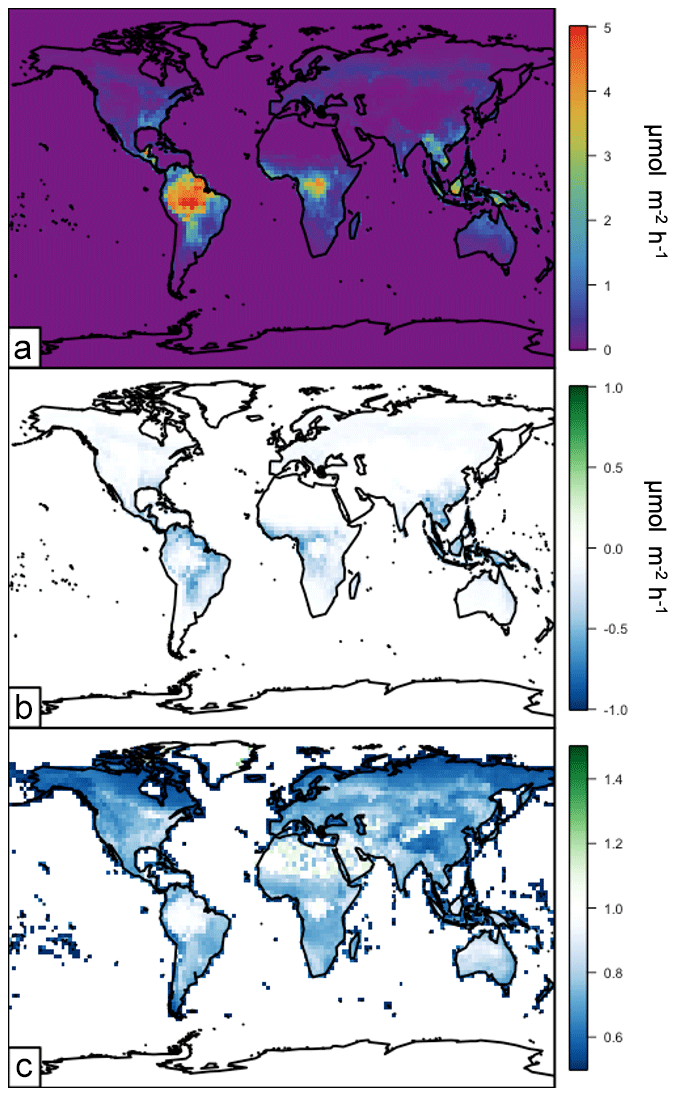
Figure 11Annual average (2012) monoterpene emissions simulated in GEOS-Chem driven by the surrogate model canopy physics. Panel (a) shows the annual average emissions. Panel (b) shows the difference between the surrogate model and the base version of simulated emissions. Panel (c) shows the relative difference between the surrogate model and the base version of simulated emissions (surrogate–base model).

Changes in simulated ozone dry deposition velocities in 2012 are summarized in Fig. 12. Figure 12a shows the annual average spatial distribution of ozone dry deposition velocities. The values vary from less than 0.1 cm s⁻¹ over the global oceans to above 0.5 cm s⁻¹ in densely vegetated regions like the tropical rainforests.

The impact of the updated canopy model on ozone dry deposition velocities is in general quite small, with an average change of near zero (∼0.004 cm s⁻¹). The annual average relative change is shown in Fig. 12b and the absolute difference in Fig. 12c, both in relation to the base version of GEOS-Chem v12.3.0. These changes are nearly all within ±5 %, or ±0.01 cm s⁻¹, with a maximum change of 15 % (0.04 cm s⁻¹). Relative changes track most strongly with broadleaf and coniferous forested areas. This is consistent with those regions being most sensitive to stomatal deposition (Silva and Heald, 2018), as the canopy scheme implemented here changes dry deposition only through the calculation of the stomatal resistance term.

Figure 12Annual average (2012) ozone dry deposition velocities simulated in GEOS-Chem when driven by the surrogate model canopy physics. Panel (a) shows the annual average dry deposition velocities (cm s⁻¹). Panel (b) shows the difference between the surrogate model and the base version of simulated dry deposition velocities (cm s⁻¹). Panel (c) shows the relative difference between the surrogate model and the base version of simulated dry deposition velocities (surrogate–base model).

The small overall changes to surface–atmosphere exchange processes associated with the updated canopy scheme produce only a modest impact on simulated atmospheric composition. We describe the changes to surface ozone here as an illustrative example.

The annual average spatial difference in surface ozone between a simulation using the canopy physics described here and the base version of GEOS-Chem is shown in Fig. 13. These changes are all generally quite small; all are within 10 % of the base simulated annual averages. The changes are generally within ±1 ppbv, with the largest absolute changes over regions with the largest changes in isoprene emissions. The distribution of differences largely follows well-known NO_x–VOC ozone formation patterns. The NO_x-limited regions of the world, in particular the remote tropics, show an inverse relationship with isoprene emissions. This is consistent with ozone titration by isoprene in the presence of low NO_x. The largest changes in ozone over the VOC-limited regimes of India and China directly correspond to the changes in isoprene emissions, with enhanced isoprene emissions over the Indian subcontinent increasing ozone concentrations and the decrease in isoprene emissions over China leading to a decline in ozone. The overall influence of the changes in ozone dry deposition velocity is fairly negligible. Even regions where the dry deposition velocity change is the largest (e.g., the Amazon) are dominated by the shift in isoprene emissions. In total, the changes in surface ozone concentrations slightly ameliorate known biases. There is a persistent high bias (∼10 ppbv) across chemical transport models in simulating surface ozone concentrations over the continental midlatitudes (Travis et al., 2016). The addition of the new canopy physics parameterization very modestly reduces this bias in GEOS-Chem (approximately 8 ppbv) by about 1 ppbv, driving simulated ozone closer to observations.

Figure 13 Annual spatial average surface ozone difference (ppbv) between the updated model version with surrogate canopy physics and the base version of GEOS-Chem (surrogate–base).

In addition to improved process representation, the canopy surrogate model presented here allows for the direct application of new emission factors generated using the MEGAN3 Emission Factor Processor (https://bai.ess.uci.edu/meganTS6, last access: 4 September 2019), which allows users to generate emission factors from various input datasets. While the focus of this work is on the impact of representing canopy physics, we include a description of this full implementation of MEGAN3 in the GEOS-Chem model for completeness. We calculate landscape-average emission factor distributions using the global growth form and ecotype distributions, the emission type speciation, and the leaf-level emission factor database available from the MEGAN3 Emission Factor Preprocessor. All MEGAN3 Emissions Factor Preprocessor options are kept at their default values (i.e., confidence rating J=0 and 20 total species classes). The land cover and emissions data are the same as those used for MEGAN2.1 except that the land cover updates described by Yu et al. (2017) were used for the contiguous US. The updated land cover is based on high-resolution (30 mm) PFT and detailed vegetation types and is expected to more accurately represent the land cover distributions in this region. The spatial distribution of the MEGAN3 activity factors is shown in Fig. 14. It is important to note that these new emission factors are input at the leaf level with units on a per LAI basis as opposed to the canopy-scale factors used in previous versions of MEGAN (applied earlier in this paper), which makes direct comparisons of emission factor magnitudes infeasible. This canopy to leaf-level change ultimately has the consequence of removing the need for the normalization factor in the activity factor calculation (see Sect. 4.1). When these emission factors are scaled to the same units as in MEGAN2.1 (i.e., the per LAI basis in the MEGAN3 emission factors is accounted for) using the MODIS LAI product applied in this work, the resulting emission factors are relatively similar (within ±75 %), though the MEGAN3 emission factors are lower than those used with MEGAN2.1 in GEOS-Chem. Generally, more than half of all changes are within 1000 $\mathrm{\mu }\mathrm{g}{\mathrm{m}}^{-\mathrm{2}}{\mathrm{h}}^{-\mathrm{1}}$, and 90 % of all emission factors are within 3000 $\mathrm{\mu }\mathrm{g}{\mathrm{m}}^{-\mathrm{2}}{\mathrm{h}}^{-\mathrm{1}}$. This comparison is not exact due to the fact that the MODIS LAI product used here is different from the input vegetation files used to create the original MEGAN2.1 emission factors. Despite the differences in absolute magnitude, the spatial patterns in emission factors in Fig. 14 are very similar to those used earlier in this work (Fig. 8), with a spatial R² of 0.91.

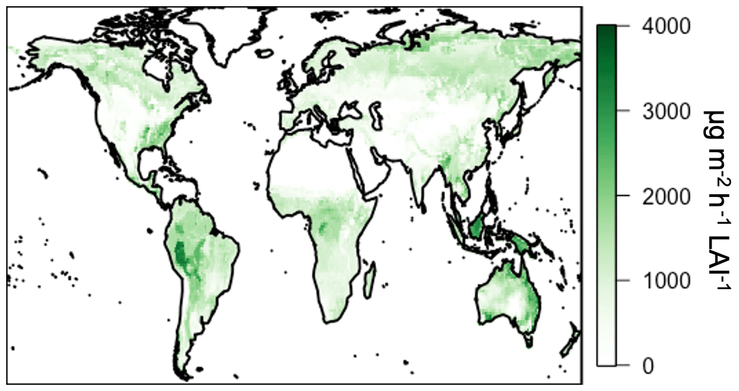
Figure 14MEGAN3 isoprene emission factors ($\mathrm{\mu }\mathrm{g}{\mathrm{m}}^{-\mathrm{2}}{\mathrm{h}}^{-\mathrm{1}}$ LAI⁻¹).

We implement the MEGAN3 emission factors in GEOS-Chem v12.3.0 using the canopy surrogate model activity factor formulation. For clarity, we refer to “MEGAN3_Full” as the emissions implementation in GEOS-Chem v12.3.0 using the MEGAN3 leaf-level emission factors and MEGAN3 activity factors with canopy physics calculated following the canopy surrogate model described in Sect. 3. The annual isoprene emissions simulated using MEGAN3_Full are higher than using the MEGAN2.1 canopy-scale factors in GEOS-Chem (as in both MEGAN_Canopy and MEGAN_PCEEA) but more in line with previous work (Guenther et al. 2012). Specifically, annual total isoprene emissions for 2012 are ∼570 Tg C yr⁻¹ in MEGAN3_Full, which is a factor of 1.6 larger than those configurations discussed earlier in this paper. The largest contribution to these differences is not the differences in emission factor maps but is instead the removal of the normalization factor of 0.21, which additionally removes the need for the somewhat arbitrary choice of “standard conditions” for emissions (see Sect. 4.1). This 570 Tg yr⁻¹ emissions total is much more similar to the magnitude of global emissions from versions of MEGAN2.1 implemented outside the GEOS-Chem model (535–578 Tg yr⁻¹) given by Guenther et al. (2012) and within the stated uncertainty range for MEGAN isoprene emissions (Guenther et al., 2012). These annual average isoprene emissions using MEGAN3_Full are shown in Fig. 15 below. In general, the spatial pattern in the emissions in Fig. 15 matches those from the MEGAN_Canopy configuration (Fig. 9), with an R² of ∼0.8.

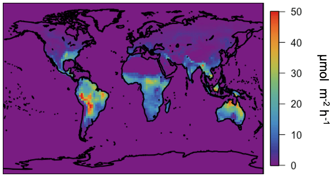
Figure 15Annual average (2012) isoprene emissions simulated in GEOS-Chem driven by the surrogate model canopy physics and the MEGAN3 emission and activity factors.

Since the isoprene emissions calculated using the MEGAN3_Full algorithm are so much larger than those used in previous versions of GEOS-Chem, they alter the composition of the atmosphere significantly. For example, annual average surface ozone concentrations in the southeastern US increase by nearly 5 ppbv relative to the base version of GEOS-Chem v12.3.0 (which uses MEGAN_PCEEA), exacerbating the existing model bias further (Travis et al., 2016). However, MEGAN3_Full represents a more up-to-date and physical characterization of biogenic emissions. Future work reconciling the differences between these bottom-up isoprene emissions estimates and top-down constraints from measurements of composition (e.g., Kaiser et al., 2018) is needed.

The MEGAN3 and GEOS-Chem model codes are available at https://bai.ess.uci.edu/megan/data-and-code (last access: 4 September 2019), and https://doi.org/10.5281/zenodo.2620535 (The International GEOS-Chem User Community, 2019), respectively. The updated GEOS-Chem code containing the canopy model changes is available at https://doi.org/10.5281/zenodo.3614062 (Silva, 2020).

CLH and SJS designed the study. SJS developed and implemented the surrogate model and performed the simulations and analysis. ABG developed the MEGAN3 model code. All authors contributed to the paper preparation.

The authors declare that they have no conflict of interest.

This research has been supported by the National Science Foundation, Division of Atmospheric and Geospace Sciences (grant no. 1564495), and the National Aeronautics and Space Administration (grant no. NNX16AN92H).

This paper was edited by Christoph Knote and reviewed by two anonymous referees.