2.1 Model description

2.1.2 Extension to regional domain

For the regional model simulation, a rotated latitude–longitude map projection with approximately 10 km horizontal grid spacing and a hybrid vertical coordinate is used. The domain of the regional model covers most of Canada and the US, as shown in Fig. 1, and consists of 528 by 708 grid points. The number of vertical levels is the same as in the global model as described in Sect. 2.1.1, namely 80 levels spanning the atmosphere from the surface to 0.1 hPa. Since the number of grid points is also almost 5 times greater than that used in the 0.9^∘ global model, the new regional model is more expensive to run. The physics packages used in the regional model are similar to those of the global model and GEM–MACH, and they include radiation (Li and Barker, 2005), boundary layer mixing (Bélair et al., 1999), shallow (Bélair et al., 2005) and deep convection (Kain and Fritsch, 1990; Kain, 2004), orographic gravity wave drag (McFarlane, 1987), and nonorographic gravity wave drag (Hines, 1997a, b) schemes. More details are provided in Mailhot et al. (1998).

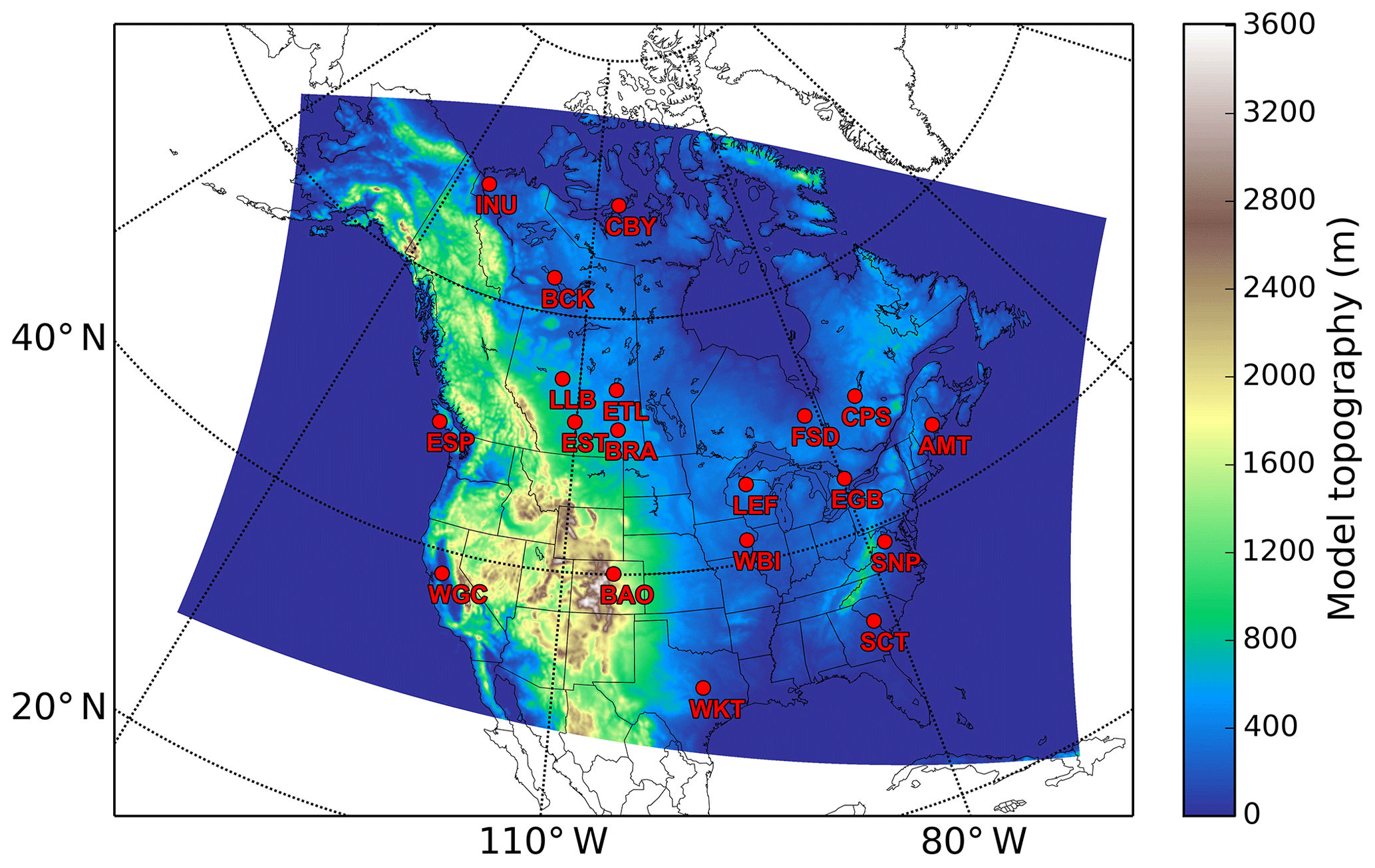
Figure 1Model topography of the regional model with 10 km horizontal grid spacing and CO₂ measurement sites used in this study (red dot with site code).

For a simulation with tagged tracers to distinguish each component of CO₂, e.g. those associated with biospheric, ocean and fossil fuel fluxes, a transport model should have the ability to simulate consistent masses across different components. In other words, the mass of the total CO₂ field should exactly equal the sum of the tagged CO₂ species, both globally and locally. This property is also required for estimating surface fluxes through Bayesian synthesis inversion (e.g. Enting, 2002). As already described in Polavarapu et al. (2016), the semi-Lagrangian advection scheme implemented in GEM alters mass slightly during model integration. The magnitude of the change for short-range forecasts is negligible, but this is not the case for the lengthy simulations of inert trace gases such as CO₂. To compensate for mass losses of tracers, a mass conservation scheme (Bermejo and Conde, 2002) and a shape-preserving locally mass-conserving scheme (Sørensen et al., 2013) were applied to tracer fields. At the lateral boundaries of the regional model domain, a mass restoration scheme (Aranami et al., 2015 scheme) is applied. These schemes, however, can make mixing ratios across multiple tracers inconsistent since they correct for global mass changes in local regions where tracer gradients are large. Since each tagged component has a rather different spatial structure and gradients from the total CO₂ field, the mass fixes made to the individual tagged variables need not be consistent with that made to the total field. As a result, the sum of each component may not equal the total CO₂ concentration field. To address this issue, the monotonicity and mass conservation schemes applied during the advection step are turned off in the regional model. The impact of the configuration on the total mass of CO₂ within the regional model domain was compared with the total mass of CO₂ from an experiment using mass-related schemes turned on. The results show that there is no significant difference between two configurations in terms of the total mass of CO₂ in the whole model domain or modelled CO₂ concentrations at the lowest model level in which most surface-based in situ observation sites are located (not shown). This occurs because the majority of tracer mass is injected into the regional model domain through its lateral boundaries. The mass of CO₂ from the surface flux is small compared to the total mass of CO₂ in the atmosphere of the regional model domain, and the signal of surface fluxes exits the lateral boundaries during model integration before they reach the upper levels of the atmosphere (e.g. upper troposphere and stratosphere). Therefore, in the regional model, we obtain perfect “additivity” of the tagged components, with a negligible loss of mass.

2.2 Surface flux

In this study, the optimised CO₂ fluxes from NOAA's CarbonTracker version CT2016 (Peters et al., 2007, with updates documented at http://carbontracker.noaa.gov, last access: 14 January 2020) were used as surface CO₂ fluxes for CO₂ simulations. The temporal resolution of the surface flux is 3 h. Because of their ready availability and careful validation, many studies aimed at global to regional to urban scales have used optimised fluxes from CarbonTracker for forward CO₂ simulations (Houweling et al., 2010; Ballav et al., 2012; Díaz-Isaac et al., 2014; Polavarapu et al., 2016; Li et al., 2017; Wu et al., 2018).

The original CT2016 flux product is available with 1^∘ by 1^∘ horizontal grid spacing. However, the global and regional models have different horizontal grid spacing. Thus, fluxes are re-gridded to GEM's grids with 0.9^∘, 0.45^∘ and 10 km horizontal spacing grid, respectively, in a mass conservative way. In addition, one more redistribution method is applied to re-gridded fluxes on the 10 km grid. This process applies a land–sea mask to the regional model grid in order to avoid unphysical modelled CO₂ concentrations caused by the different behaviour of vertical mixing over land and water grid cells. Because coarse-resolution fluxes do not contain all the information needed for high-resolution grid cells, considering only the size of a grid cell in re-gridding is insufficient because it would lead to modelled CO₂ concentrations that are too low or too high relative to observed CO₂ concentrations in regions of strong surface CO₂ fluxes. With respect to fossil fuel emissions, for example, dynamic consistency is one of the important factors in regional-scale CO₂ concentration simulations, in particular along coastal margins (Zhang et al., 2014). Hence, biospheric and fossil fuel flux components on water grid cells in which the fraction of land is less than 30 %, including lakes and oceans, are redistributed into land grid cells (within a radius of 30 grid points) in order to simulate realistic CO₂ concentrations along coastlines in the regional model domain while minimising the impact of redistributed surface fluxes on CO₂ simulation and while conserving the total mass of surface fluxes within the regional model domain.

2.3 Observations

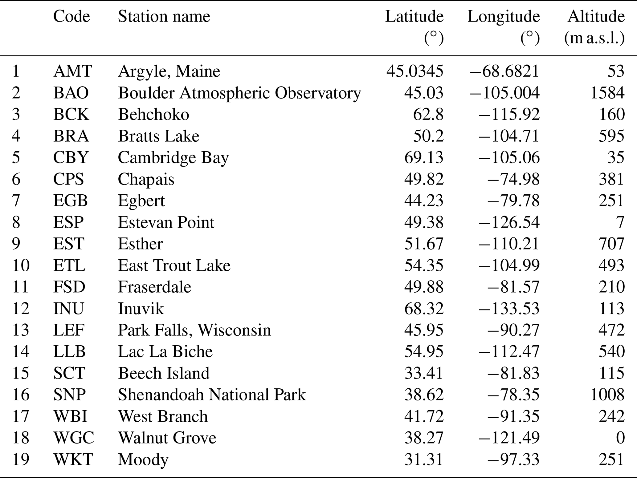
Modelled CO₂ concentrations are verified against observations from ObsPack (Masarie et al., 2014), which is maintained and provided by NOAA. For surface measurement sites, not all observations available in the regional model domain are used in the evaluation. The following selection criteria are applied: (1) sites were used to infer optimised CO₂ fluxes in CT2016. Thus, we can expect that optimised surface fluxes from CT2016 provide information about sources and sinks consistent with observed CO₂ concentrations at those sites so that differences in model simulation results may be attributable to model error. (2) Sites have continuous measurements (e.g. hourly data), as we want verify the results for all forecast hours. (3) Sites have no periods of missing data longer than 1 month (except for ESP – see Table 1 for a full list of station abbreviations – which has no data in January 2015), so results can be obtained for all seasons during the experimental period. As a result, 19 measurement sites (11 sites in Canada and 8 tower sites in the US) are selected as shown in Fig. 1 and listed in Table 1. For aircraft profiles of CO₂, measurement sites available over Canada and the US in the year 2015 were selected.

Table 1Information for surface in situ measurement sites used in this study.

Download Print Version | Download XLSX

2.4 Experiment design

Three experiments are performed as listed in Table 2. GLB90 is the reference experiment using the global model with 0.9^∘ horizontal grid spacing. GLB45, which uses the global model with 0.45^∘ horizontal grid spacing, is carried out to provide LBCs to the regional model. LAM is the regional model run with 10 km horizontal grid spacing. The simulation period is 1 year for 2015. In the analysis, the first 10 d of simulations are regarded as a spin-up period and discarded.

Table 2Experiment design. n/a – not applicable

Download Print Version | Download XLSX

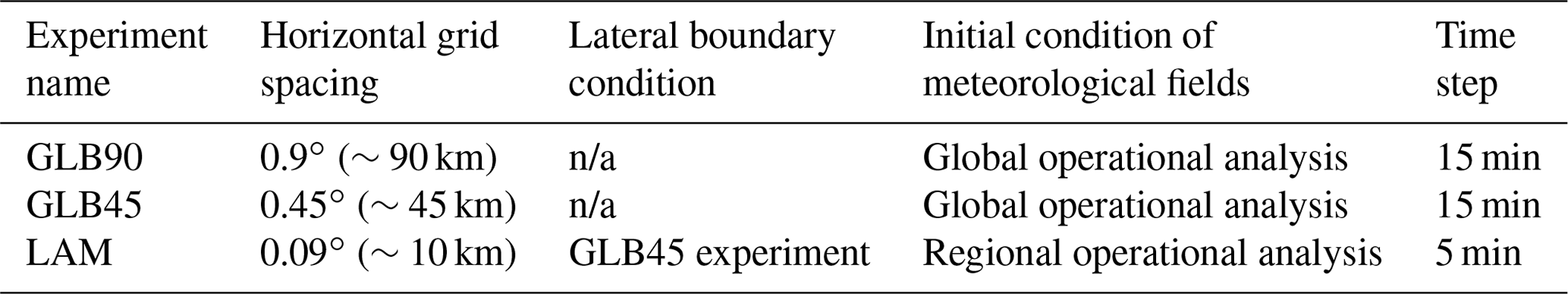
Figure 2 depicts the global and regional model cycles. In each forecast, the weather forecast and CO₂ transport by forecasted wind fields are performed simultaneously at every time step. For the initial condition (IC) of meteorological fields for the two global models at the beginning of every cycle, the operational global analysis products from the global deterministic prediction system (GDPS; Buehner et al., 2015), whose horizontal resolution is roughly 25 km on a regular latitude–longitude grid or, as of 15 December 2015, a yin–yang grid (Qaddouri and Lee, 2011), are used. The archived data are interpolated to our low-resolution grids and topographies of GLB90 and GLB45 separately. For the IC of meteorological fields for the regional model, the operational regional analysis products from the regional deterministic prediction system (RDPS; Fillion et al., 2010; Caron et al., 2015) are used. The regional model grid is a subset of the model domain of the operational RDPS with the same horizontal resolution, sharing grid points on the same latitudes and longitudes. Therefore, it is not necessary to perform a horizontal interpolation at the start of every cycle. Also, a spin-up period for the meteorological forecast is unnecessary. Both operational global and regional meteorological analyses are produced four times per day with a 6 h assimilation window centred on the analysis time. We only use analyses produced at 00:00 UTC every day as an IC of meteorology. Thus, a 24 h weather forecast is produced during each 24 h CO₂ cycle, and these forecasts are replaced by new analyses at every 00:00 UTC, with the exception of microphysics tracers which are retained to allow a hot start for the hydrometeor fields (Milbrandt et al., 2016). On the other hand, the mass of CO₂ in a model grid volume is kept during cycles without replacements. The 24 h forecast of CO₂ from the previous cycle is used as the IC of the CO₂ field for the next cycle at 00:00 UTC. This is combined with the updated meteorological analysis for a complete initial state for the coupled model. Such 24 h forecast cycles are also used in other global model systems (e.g. Agustí-Panareda et al., 2014; Ott et al., 2015).

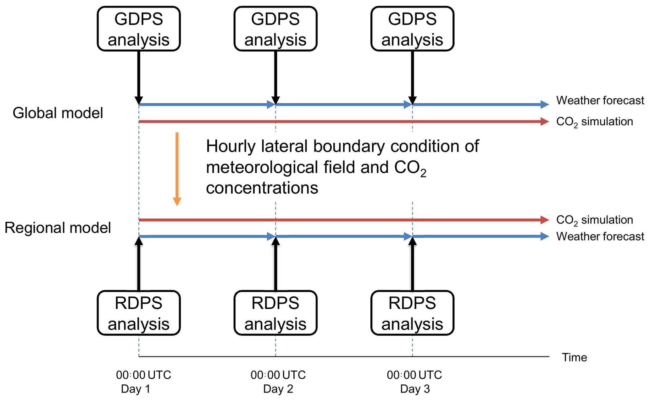
Figure 2Schematic diagram of GEM–MACH–GHG global and regional forward model cycles. Meteorological analyses are from CMC's operational global deterministic prediction system (GDPS) and regional deterministic prediction system (RDPS). Global and regional 24 h weather forecasts start at 00:00 UTC each day with operational analyses, while CO₂ concentrations are kept during cycles. The global forward model provides the lateral boundary condition of meteorological and CO₂ fields to the regional forward model every hour.

Download

The IC of 3-D atmospheric CO₂ concentrations at the beginning of all three experiments is taken from CT2016 CO₂ concentrations at 00:00 UTC on 1 January 2015. The LBC of CO₂ concentrations for the regional model are obtained from GLB45 and include hourly meteorological and CO₂ fields.

One more possible configuration is using operational RDPS forecasts as meteorological LBCs for the regional model, which is similar to the configuration of the operational regional GEM–MACH (Moran et al., 2010). We tested this configuration and compared modelled CO₂ concentrations with the LAM experiment's modelled CO₂ concentrations. A negligible difference was found (not shown), and therefore we decided not to include that configuration in this study because our purpose is to develop an integrated global–regional forward modelling framework for GHG simulations as shown in Fig. 2.

2.5 Sampling method and metrics

In order to evaluate the performance of CO₂ simulations and meteorological forecasts, a series of metrics are used as described below. Modelled or forecasted values are sampled at the observed location by applying horizontal and vertical interpolation to model fields rather than selecting the nearest grid point to measurement locations and selecting the time step closest to the observed time. To sample modelled CO₂ concentrations, the sampling height above the ground level (or the model surface level) is considered to determine the altitude for vertical interpolation instead of using the actual sampling height above sea level (i.e. the sum of the altitude of an observation site plus intake height). Coarse-horizontal-resolution models cannot resolve the complex topography well (e.g. mountain regions) around some measurement sites. As a result, the altitude of model topography may be far above or below the actual height of a measurement site. If the height of a model-sampled observation is erroneously placed in the PBL (free troposphere) as a result of coarse model topography, this can result in an unphysical diurnal cycle of CO₂ that is too strong (too weak) compared to observed values (see Agustí-Panareda et al., 2019). From a comparison of the two sampling methods, it was found that the LAM experiment is not sensitive to the vertical sampling method, as expected, because it can resolve actual topography well thanks to the higher spatial resolution, but the GLB90 experiment is sensitive to the method at a number of measurement sites (not shown). Thus, in order to reduce the topography mismatch problem in the coarse-resolution global model and investigate the impact of higher horizontal resolution without this problem, the method using intake height is used to help the global model capture the behaviour of the PBL variations with time and height. A detailed discussion of the vertical sampling methods in connection with horizontal resolution is found in Agustí-Panareda et al. (2019).

To analyse our results, including CO₂ and meteorology, the bias and standard deviation of forecast error (SD) are used.

The bias is defined as

where N indicates the number of observations, M_i indicates modelled CO₂ concentration or meteorological forecast, and O_i indicates the corresponding observation. The SD is defined as

where $X_i=M_i-O_i$ and the overbar refers to the bias of the quantity.

To calculate the amplitude of the CO₂ diurnal cycle (or other frequencies) for a measurement site or grid point, we use a discrete Fourier transform (DFT) technique. The linear trend in hourly CO₂ time series from a specific location is removed first, and then the DFT technique is applied to the detrended CO₂ time series to extract the amplitude of CO₂ variability across temporal scales, from synoptic to diurnal to sub-daily scales, as discussed in Sect. 4.4.

3.1 Evaluation of meteorological fields

Before considering CO₂ simulation results, weather forecasts from the three experiments are verified against observations over the regional model domain and are compared with each other. The motivation for doing this is two-fold: (1) to check that the meteorological forecasts from our regional model have not drifted away from the operational forecasts, which have been produced and maintained by the CMC for many decades, and (2) to compare the regional model results with the global model results. The first check is necessary because the configuration for weather prediction and the GEM model version used in this study are different from what was used to produce the operational forecast in 2015. For example, LBCs in RDPS were obtained from a global model forecast using a 33 km horizontal grid spacing (Caron et al., 2015) (or with a 25 km horizontal grid spacing as of 15 December 2015), with a different model domain extent and vertical coordinate. As shown by Polavarapu et al. (2016), the performance of the weather forecast by the global model is already well evaluated. The uncertainty of 24 h weather forecasts in the global model corresponding to the GLB90 experiment in this study is comparable with those of reanalyses provided by three operational centres; the monthly and zonal means of fields in 2009 and 2010 are within an acceptable range on global scales. Thus, in this section, we focus on the regional model results and on differences between experiments in the regional domain.

Figure 3 shows the bias and SD of the 24 h forecast error for the three experiments for vertical levels from 1000 to 10 hPa in July 2015. The same numbers of North American radiosonde observations are used in each of the three sets of verifications, and these are indicated on the right of each panel. The statistical significance of the differences using a T test for the means or an F test for the standard deviations at the 95 % confidence level was computed but is not shown explicitly. However, the discussion below uses this information in that we only mention results that are statistically significant. The three experiments show good agreement with observations in terms of bias and SD. For zonal wind, there are quite small differences among experiments, and the scores remain within the range of operational forecasts (not shown), except at 925 and 850 hPa where biases in the GLB90 and GLB45 experiments are slightly better than those in the LAM experiment (Fig. 3a). For wind speed, unlike the zonal wind, forecasts in the LAM experiment are better than those from the GLB90 experiment for levels from 925 to 50 hPa and better than those in the GLB45 experiment for levels from 300 to 70 hPa and at 700 hPa (Fig. 3b). For geopotential height, the forecasts in the LAM experiment are better than those in the GLB90 and GLB45 experiments from 400 to 10 hPa where relatively large positive biases in the GLB90 and GLB45 experiments exist. In addition, the SD in the LAM experiment is better at all vertical levels except a few levels (Fig. 3c). For temperature, the forecasts in the LAM experiment are better than those in the GLB90 and GLB45 experiments from 1000 to 70 hPa, with the exception of 150 hPa (Fig. 3d).

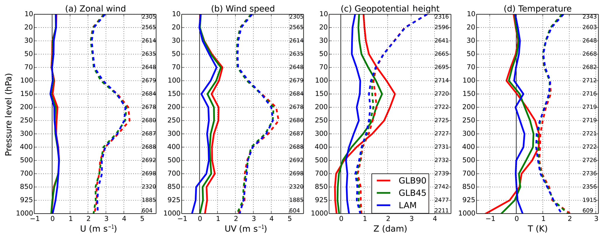
Figure 3The bias (solid line) and standard error (dashed line) of (a) zonal wind (m s⁻¹), (b) wind speed (m s⁻¹), (c) geopotential height (dam) and (d) temperature (K) from the GLB90 (red), GLB45 (green) and LAM (blue) experiments based on a comparison the 24 h forecasts against North American radiosondes for July 2015. The numbers on the left side of each panel denote the pressure level. The numbers on the right side of each panel denote the number of observations used in the statistics at each pressure level.

Download

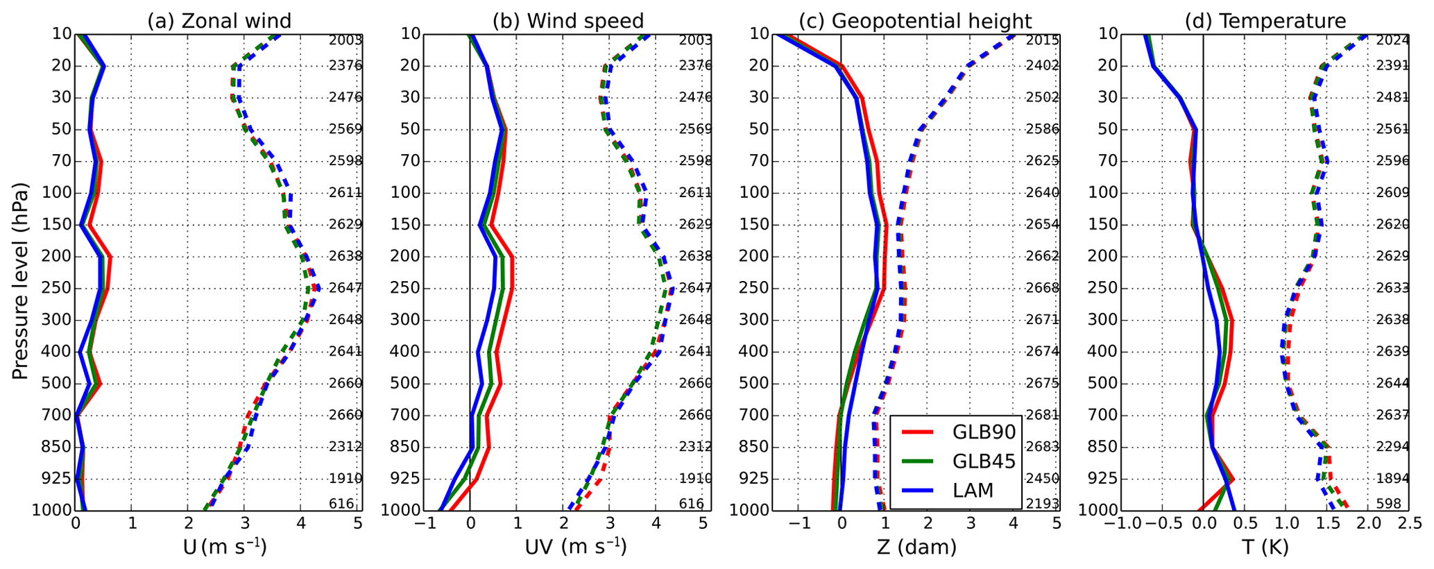
The scores for December 2015 are shown in Fig. 4. The differences in bias and SD among experiments are smaller than those in July. In addition, patterns in the reduction of bias and SD from coarse horizontal resolution to higher horizontal resolution can be seen much more clearly than in July, which means that the values in the GLB45 experiment are located between those of the GLB90 and LAM experiments. For zonal wind, there are quite small differences in bias and SD among experiments, as was the case in July (Fig. 4a). For wind speed, forecasts in the LAM experiment are better than those in the GLB90 experiment from 850 to 150 hPa as well as those in the GLB45 experiment at 500 and 400 hPa but not better at 925 hPa (Fig. 4b). For geopotential height, both bias and SD in the LAM experiment are better than those in the GLB90 experiment at most pressure levels except from 700 to 400 hPa, while the LAM experiment is better than GLB45 from 1000 and 925 hPa (Fig. 4c). For temperature, the bias in the LAM experiment is better than that in the GLB90 and GLB45 experiments from 925 to 250 hPa (Fig. 4d).

Figure 4As in Fig. 3, but for December 2015.

Download

It is also worth considering how our meteorological forecasts compare to those of other systems. Agustí-Panareda et al. (2019) show root mean square errors (RMSEs) of vector wind for January and July 2014 from 1 d forecasts from the Copernicus Atmosphere Monitoring Service (CAMS). Our RMSE scores computed using the data from Figs. 3 and 4 for wind speed are shown in Table S1 in the Supplement, and these can be compared to their Fig. 4. Our LAM scores are lower than those of the 9 km CAMS at all heights in January and July. However, this is not a fair comparison since their scores are for a global domain, whereas we consider the North American domain, and their values are for 2014 but ours are for 2015. Nevertheless, the comparability of the scores further suggests that our LAM is performing well in terms of 24 h meteorological forecasts.

The number of available observations at 1000 hPa is much smaller than that of other pressure levels (see the numbers on right side of each panel in Figs. 3 and 4); because the typical altitudes of many sites are above the level corresponding to 1000 hPa and surface pressures may be below 1000 hPa depending on the synoptic situation, there is little confidence in the verification at this level by means of radiosondes. A better approach to rigorously investigate the performance of weather forecasts at lower levels is to use surface observations because of their much greater numbers (in both space and time). Therefore, weather forecasts in the three experiments are also verified against observations near the surface. Figure 5 shows the bias and SD of sea level pressure, 2 m temperature and 10 m wind speed as well as the Heidke skill score (HSS) (Wilks, 2006) of 10 m wind direction for July 2015. The SD of sea level pressure in the LAM experiment is lower than those in the GLB90 and GLB45 experiments, while the bias of sea level pressure in the LAM experiment is slightly lower than those of the GLB90 and GLB45 experiments. However, the difference between the LAM and the GLB90 and GLB45 biases does not exceed 0.5 hPa (Fig. 5a). The SDs of 2 m temperature and 10 m wind speed in the LAM experiment are smaller than those in the GLB90 and GLB45 experiments for all forecast hours (Fig. 5b and c), which implies that the error of forecasts from the LAM experiment fluctuates less than those of the GLB90 and GLB45 experiments. Also, the better results of the LAM experiment in 10 m wind direction is evident in the higher HSS of the LAM experiment (Fig. 5d). Higher HSS means a better forecast of wind direction. In addition, the root mean square errors (RMSEs) of variables in the LAM experiment are lower than those of the GLB90 and GLB45 experiments (not shown).

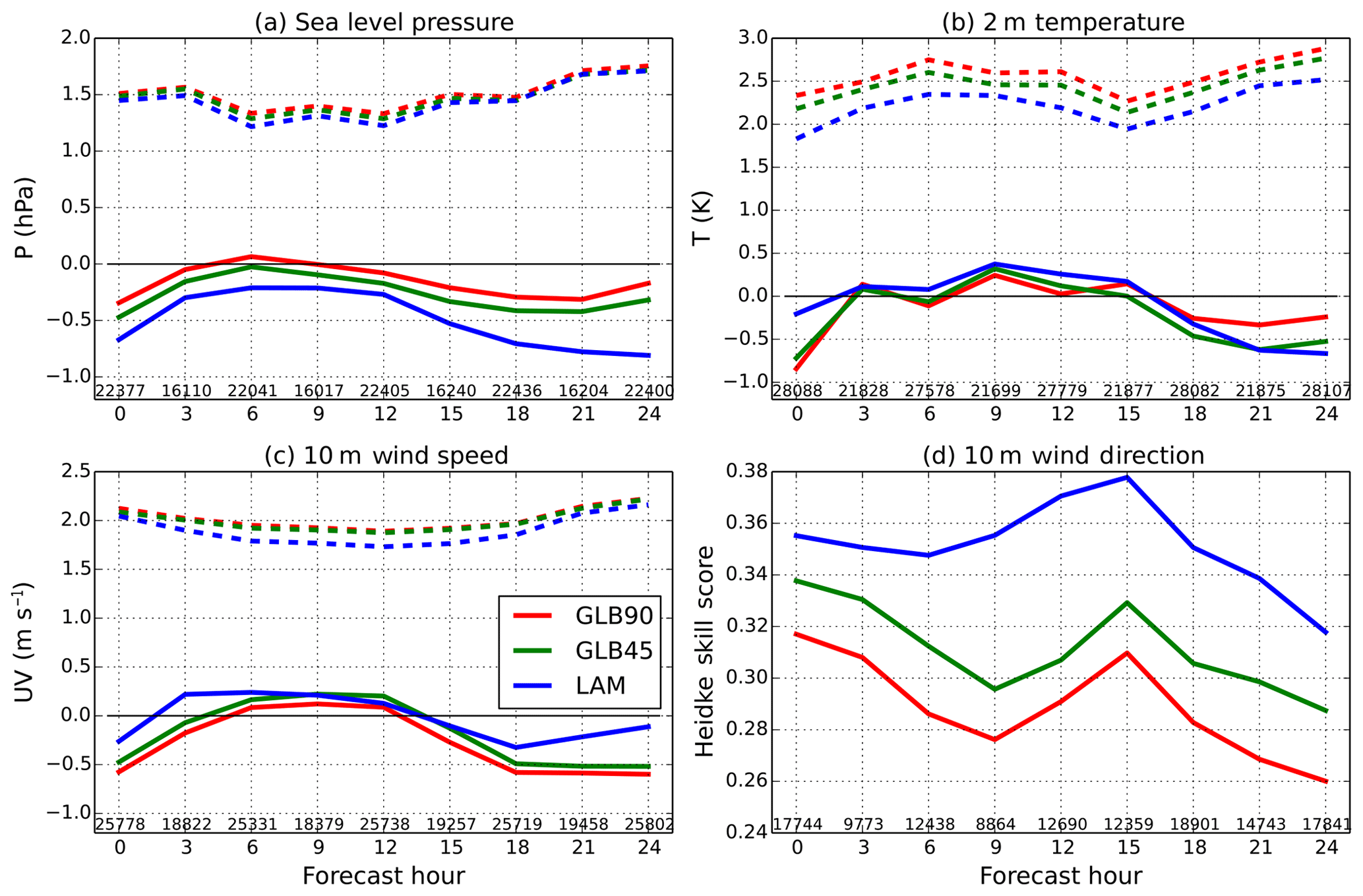
Figure 5The bias (solid line) and standard error (dashed line) of (a) sea level pressure (hPa), (b) 2 m temperature (K), (c) 10 m wind speed (m s⁻¹) and (d) Heidke skill score of 10 m wind direction from the GLB90 (red), GLB45 (green) and LAM (blue) experiments based on a comparison of forecasts against surface-based stations over North America for July 2015. The numbers at the bottom of each panel denote the number of observations used in the statistics at each forecast hour.

Download

In December 2015, the better forecasts in the LAM experiment compared to those of the GLB90 and GLB45 experiments can be seen more clearly (Fig. 6). The bias and SD of each variable in the LAM experiment are lower than those of the GLB90 and GLB45 experiments at most forecast hours (Fig. 6a–c), and higher HSS values of 10 m wind direction are evident at all forecast hours (Fig. 6d).

Figure 6Same as Fig. 5, but for December 2015.

Download

In summary, the LAM experiment produces reasonable meteorological forecasts in comparison with meteorological observations and better results relative to the GLB90 and GLB45 experiments, in particular at surface levels which are important for correctly capturing the flow of CO₂ affected by surface fluxes and boundary layer mixing, with reductions in both bias and SD. Since forecasted meteorological fields are used to transport CO₂ in each simulation individually, better CO₂ simulations in the LAM experiment can be expected in the verification of modelled CO₂ concentrations.

3.2 Evaluation of CO₂ fields

The CO₂ fields in the LAM and other experiments are investigated in terms of the monthly bias and SD of daily afternoon (12:00–16:00 LST) modelled CO₂ concentrations at the measurement sites shown in Fig. 1 and listed in Table 1 (Fig. 7). Daily afternoon time was selected because this is what CT2016 used to estimate surface CO₂ fluxes. Also, CT2016 results are included as a reference since this is what all our model experiments used as input fluxes. In general, bias and SD in summer are larger than in other seasons at most sites except BAO, SCT, WGC and WKT. Better results in CT2016 than in all three experiments at many sites can be seen, especially in June to October. Surface CO₂ fluxes from CT2016 were inferred by minimising the difference between observations and forecasts of TM5 (Krol et al., 2005), which is the transport model used in CT2016. CT2016 fluxes thus contain an imprint of TM5's transport so that when GEM–MACH–GHG is forced with CT2016 fluxes, the mismatch of transport between the two models is evident (Polavarapu et al., 2016). As a result, larger biases in the three experiments relative to CT2016 at the abovementioned sites may be expected due to the discrepancies of modelled CO₂ concentrations between CT2016 and GEM–MACH–GHG. In contrast, the three models show similar biases to each other except at ESP and WGC, especially in boreal summer. Since the LAM experiment uses LBCs of CO₂ concentrations from the GLB45 experiment, information about the large-scale transport of the CO₂ concentration is reflected in LAM experiment.

Figure 7Monthly mean bias of daily afternoon averaged (12:00–16:00 LST) CO₂ concentrations from the GLB90 (red), GLB45 (green) and LAM (blue) experiments as well as CT2016 (cyan) at all measurement sites used in this study.

Download

Now we consider the seasonal variation of the performance of the LAM experiment over the regional (North American) domain. The seasonal bias and SD of modelled CO₂ concentrations in the LAM experiment are shown in Fig. 8 based on daily afternoon CO₂ concentrations. In boreal winter (DJF) and spring (MAM), there are mainly positive biases at most Canadian sites, while SDs are small relative to other sites in the US. The magnitude of surface CO₂ fluxes in those seasons over Canada is quite small (not shown), and thus bias at the Canadian sites contributes little to the overestimation of CO₂ concentrations. This result suggests that biases included implicitly in the LBC of CO₂ concentrations provided by the GLB45 experiment are more important in determining the biases in the regional model domain in those seasons. Four sites (BRA, EST, ETL and LLB) in Alberta and Saskatchewan show relatively large SD in DJF due to local influences of surface fluxes trapped within a shallow boundary layer by low temperatures. On the other hand, in boreal summer (JJA), large SD can be seen with negative biases at most sites. The large biases and SD in JJA may be attributed to errors in terrestrial CO₂ fluxes within the regional model domain. As shown in Fig. 7, the GLB90 and GLB45 experiments underestimate CO₂ concentrations over northern sites in JJA. That is also reflected in the underestimation of CO₂ concentrations in the LAM experiment because the same surface fluxes are used in the simulations. Finally, in boreal autumn (SON), both biases and SD show moderate values between MAM and JJA. Negative biases at northern sites in the LAM experiment are partially due to biases in the LBCs obtained from the GLB45 experiment. In summary, the performance of the regional model partially depends on biases in the global model which provides the LBC, and the relative importance of these biases varies with season. In this regard, the use of CT2016 posterior fluxes to drive our global models exacerbates such biases. However, in the future when our global models provide their own flux estimates, such biases may be reduced. Furthermore, the need for a better understanding of the relative role of initial and boundary conditions and surface fluxes in controlling CO₂ distributions within the regional model domain is evident. This is the subject of our future work.

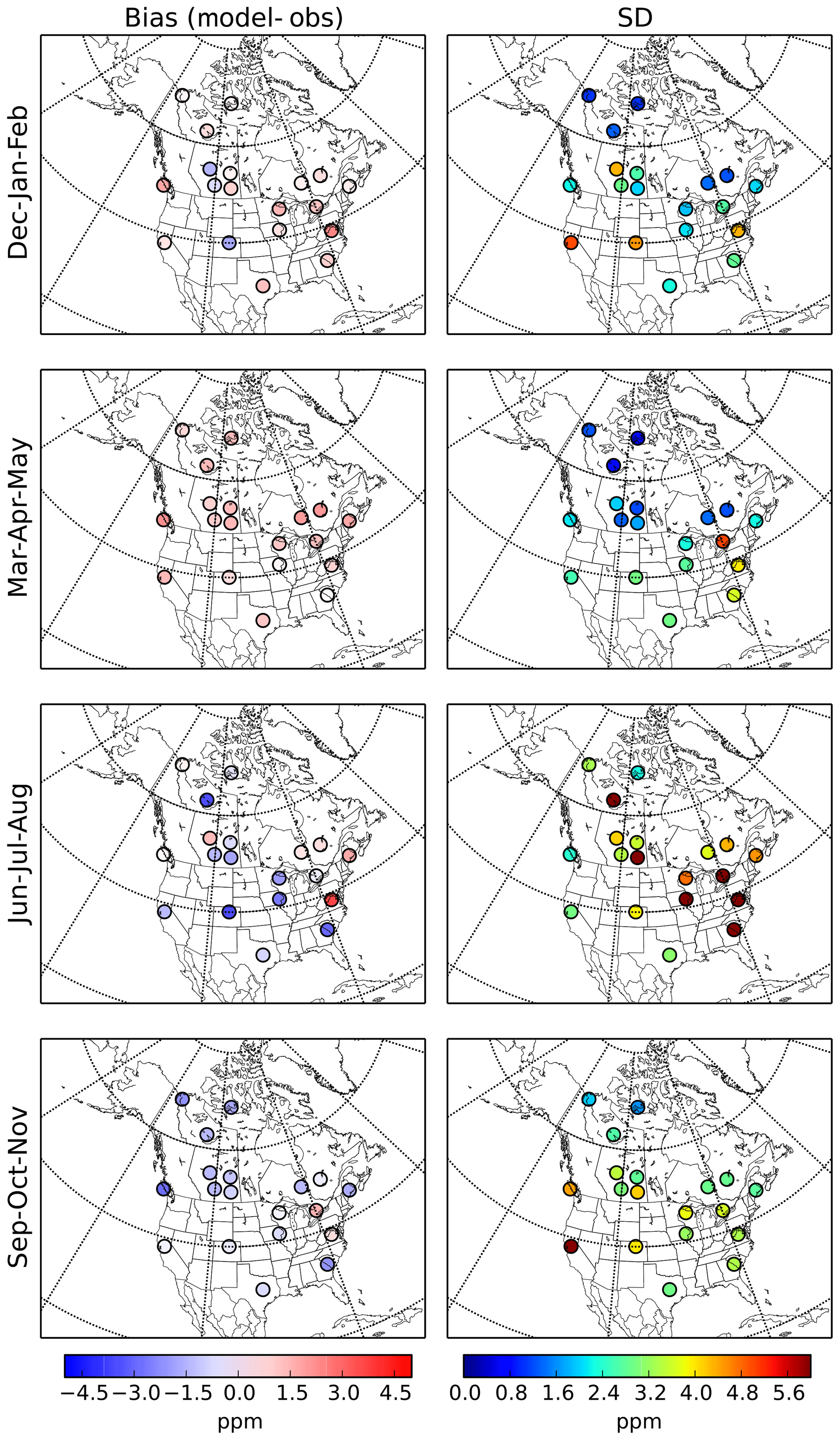
Figure 8Mean (left column) and standard deviation (right column) of the residuals between modelled CO₂ from the LAM experiment and observed CO₂ concentrations (modelled – observed) at each observation site over January to February and December 2015 (first row), March to May 2015 (second row), June to August 2015 (third row), and September to November 2015 (fourth row).

4.1 Spatial patterns of surface CO₂ concentrations

Biases between two experiments are compared pairwise for four seasons (Fig. 9). Three comparisons are shown because three experiments are conducted. Since bias can have both positive and negative values, absolute bias is used in the calculation. Blue (red) means that the higher-horizontal-resolution model simulated smaller (larger) absolute bias compared to the coarser one. In DJF, the GLB45 and LAM experiments are better than the GLB90 experiment. However, the LAM experiment is not better than the GLB45 experiment at US sites except WGC and BAO. In MAM, the differences among the experiments are the smallest, except at ESP near the west coast of North America. Differences between the LAM and GLB45 experiments at northern Canadian sites are quite small in DJF and MAM, which is associated with weak surface CO₂ fluxes in those seasons. In JJA, the reduction in bias resulting from the higher-horizontal-resolution model can be seen clearly, and the magnitude of the reduction is higher, probably due to better weather simulation (less transport error) as shown in Figs. 3, 4, 5 and 6. The LAM experiment shows better results than both the GLB90 and GLB45 experiments at most sites. On the other hand, the GLB45 experiment is not better than the GLB90 experiment except at a few sites. This nonlinearity of the improvement with increased resolution is consistent with the results of Agustí-Panareda et al. (2019), although their conclusions are based on RMSE rather than absolute bias. In SON, the results are similar to those in JJA; namely, the LAM experiment is better than both the GLB90 and GLB45 experiments at most sites except ESP. At many sites, the benefit of finer grid spacing is evident, but higher horizontal grid spacing does not always guarantee a lower magnitude of bias for all sites. Part of the reason that improvement is not clear at certain sites in Fig. 9 may be due to the focus on afternoon mean values. For example, if we consider higher-temporal-frequency output (i.e. hourly residuals), LAM is better than GLB90 and GLB45 even at ESP in November (Fig. S1 in the Supplement).

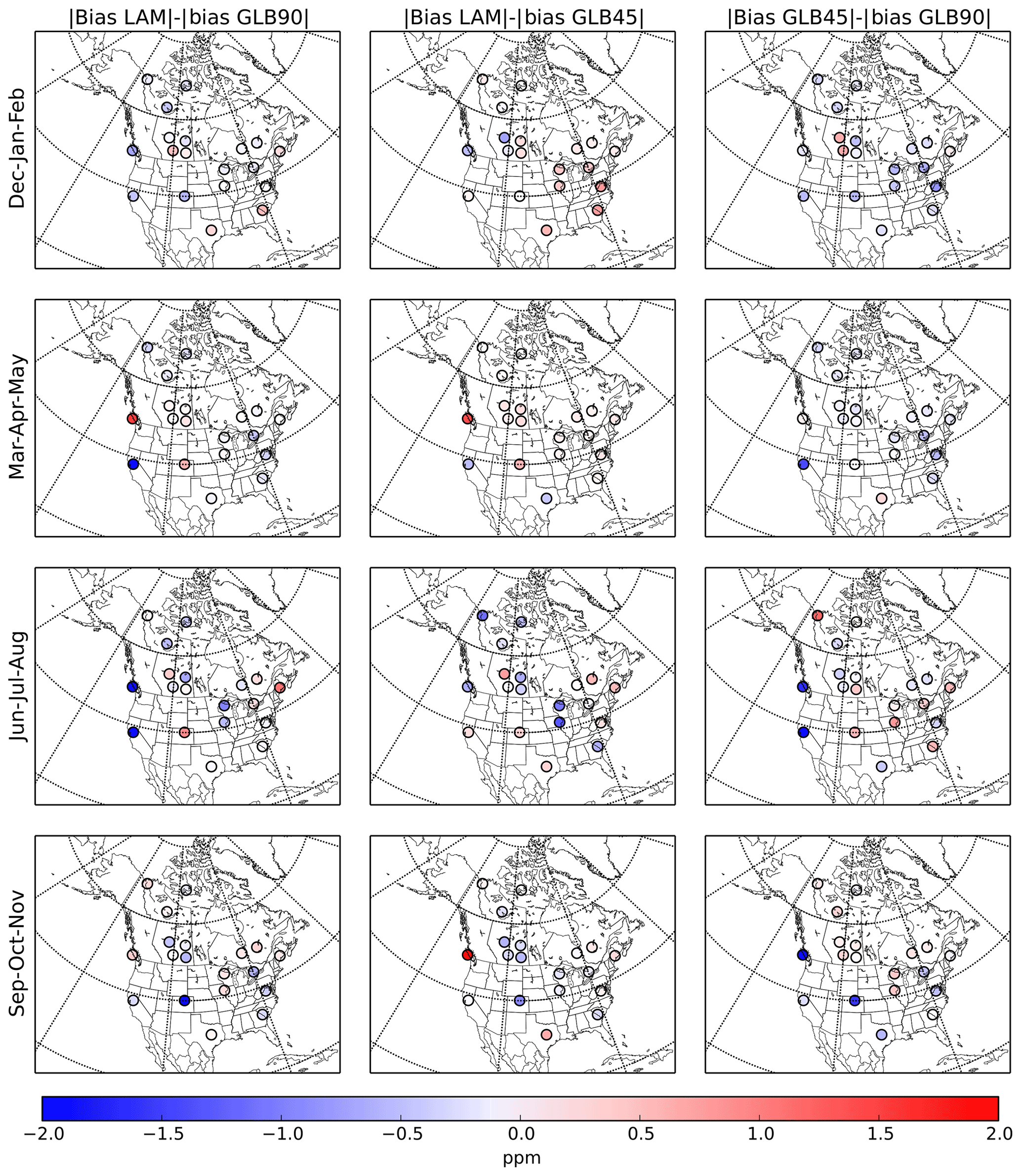
Figure 9The difference in absolute mean bias between GLB90 and LAM (first column), GLB45 and LAM (second column), and GLB90 and GLB45 (third column) over January to February and December 2015 (first row), March to May 2015 (second row), June to August 2015 (third row), and September to November 2015 (fourth row).

Figure 10 shows the differences in SD between two experiments. The spatial pattern of differences in SD is different from that of bias. More blue dots are evident, indicating that the SD of the higher-horizontal-resolution model is smaller than that of the coarser-horizontal-resolution model at most sites. Specifically, the LAM experiment shows better results than both the GLB90 and GLB45 experiments in DJF. As shown in Fig. 6c and d, better forecasts of 10 m wind speed and direction at screen level in the LAM experiment should help to reduce SD in the LAM experiment relative to the two global model experiments. In MAM, the impact of horizontal resolution is very small at most sites except near the southern boundary of the regional model domain due to the weak magnitude of the surface CO₂ flux in this season. The ratio between CO₂ concentrations resulting from surface CO₂ fluxes within the regional model domain and background CO₂ concentrations from the GLB45 experiment shows that the contribution of the surface CO₂ flux is the lowest in MAM due to the small magnitude of the surface CO₂ flux (not shown). In JJA, on the other hand, the magnitude of the difference is larger than in other seasons in both positive and negative directions. Finally, in SON, the improvement due to finer grid spacing can be seen.

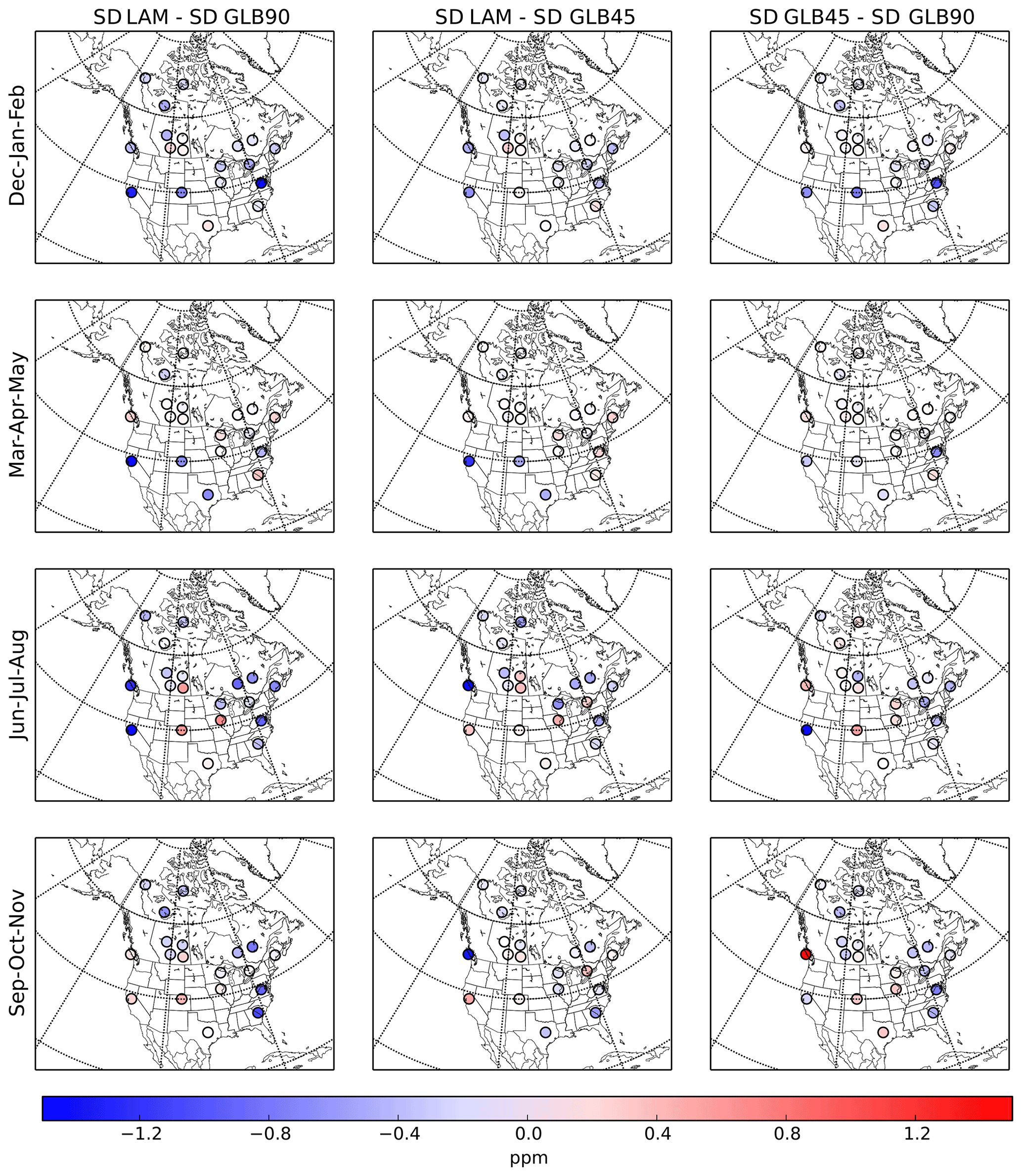
Figure 10The difference in the standard deviation of the residuals between modelled CO₂ and observed CO₂ concentrations (modelled – observed) between GLB90 and LAM (first column), GLB45 and LAM (second column), and GLB90 and GLB45 (third column) over January to February and December 2015 (first row), March to May 2015 (second row), June to August 2015 (third row), and September to November 2015 (fourth row).

In summary, the differences in bias and SD between experiments provide evidence of improvement in CO₂ simulations due to finer horizontal resolution and better wind forecasts near the surface in the LAM experiment. The pattern of the differences is strongly associated with the spatial and seasonal patterns of the magnitude of surface CO₂ fluxes used in the simulations.

4.2 Vertical profile of CO₂ concentrations

We now consider the quality of modelled CO₂ concentrations in the free troposphere. Observed profiles of CO₂ can reveal the signatures of vertical mixing, so they can be used to measure the performance of transport models (Lin et al., 2006). The seasonal bias and SD of vertical profiles of modelled CO₂ concentrations against NOAA aircraft profiles (Sweeney et al., 2015) over sites in Canada and the US inside the regional model domain are shown in Fig. 11. Modelled CO₂ concentrations are sampled at the exact location and height of observations by applying vertical and horizontal interpolation to 3-D model fields at a time step close to the observed time. Then, averages over all profiles of modelled and observed values for a season are binned into 1 km thick layers. The three experiments generally overestimate CO₂ concentrations in DJF (at 1000 m) and MAM and underestimate them in JJA and SON, which is consistent with the comparisons against surface CO₂ measurement sites shown in Fig. 8. The magnitude of the bias does not exceed about 2 ppm in any altitude or season, and it decreases with altitude. Profiles of CO₂ concentrations near the ground are difficult to simulate due to the strong influence of surface fluxes (Geels et al., 2007). The range of the biases in the three experiments is similar to that seen in our previous study (Polavarapu et al., 2016) as is the direction of the biases. Specifically, the bias changes sign with height, with positive biases at low altitudes and negative biases in DJF and MAM. In JJA and SON, the bias remains negative at almost all heights. The LAM experiment generally has the smallest biases for all seasons and altitudes, in particular below 4000 m in JJA when the influence of surface CO₂ fluxes is significant through active vertical mixing. Lower wind speeds in boreal summer compared to other seasons causes the accumulation of surface fluxes over North America in the lower 4000 m (Sweeney et al., 2015). Reduced bias and SD of forecasted temperature profiles in the LAM experiment in July (Fig. 3d) may help to improve vertical advection in the LAM simulations relative to the global model experiments through improved buoyancy calculations. This may explain why the LAM experiment has a better ability to simulate vertical profiles of CO₂.

Figure 11Comparison of profiles of modelled CO₂ concentrations from the GLB90 (red), GLB45 (green) and LAM (blue) experiments to NOAA aircraft observations for (a) January to February and December 2015, (b) March to May 2015, (c) June to August 2015, and (d) September to November 2015. Solid line denotes mean bias and dashed line denotes standard error. The sites used are as follows: Briggsdale, Colorado; Cape May, New Jersey; Dahlen, North Dakota; Estevan Point, British Columbia; East Trout Lake, Saskatchewan; Homer, Illinois; Park Falls, Wisconsin; Worcester, Massachusetts; Poker Flat, Alaska; Charleston, South Carolina; Southern Great Plains, Oklahoma; Sinton, Texas; Trinidad Head, California; West Branch, Iowa.

Download

4.3 Temporal patterns

We evaluate modelled CO₂ concentrations at various temporal scales including synoptic variability and the diurnal cycle. First, the synoptic variability of modelled CO₂ concentrations is analysed. Figure 12 shows Taylor diagrams (Taylor, 2011) of modelled CO₂ concentrations in the afternoon compared with observations. Since the domain of the LAM experiment covers a variety of geographic regions across Canada and the US, including mountain, continental and coastal sites, the synoptic variability of CO₂ is not expected to be captured well at all sites. In DJF, the variability of modelled CO₂ concentrations in the LAM experiment is closer to the observed variability than that captured in the GLB90 and GLB45 experiments, in accordance with the decreased SD seen in Fig. 10 (Fig. 12a). In MAM, the variability of modelled CO₂ is scattered, with relatively lower correlations than other seasons (Fig. 12b). In general, due to the onset of the growing season in MAM, transport models tend to produce lower correlations with observed CO₂ (Geels et al., 2004; Pillai et al., 2011; Agustí-Panareda et al., 2014). In JJA, despite having larger biases than other seasons (Fig. 7), correlations are quite reasonable, mostly lying between 0.6 and 0.95 (Fig. 12c). However, the variability in the CO₂ concentrations tends to be overestimated. This could be mainly due to the large uncertainty in biospheric fluxes (Patra et al., 2008). Also, the range of correlations is the biggest – between approximately 0 and 0.95. In SON, the synoptic variability of CO₂ is well captured by all experiments (Fig. 12d). Many sites have correlations higher than 0.9, standard deviations similar to observed variability and the least normalised RMSE (the distance from the reference point on the x axis) relative to other seasons. We expect the LAM experiment to produce higher correlations and smaller normalised RMSEs, as well as normalised standard deviations approaching 1. Indeed, the LAM experiment tends to simulate the observed variability of CO₂ well, and it produces a smaller normalised RMSE relative to the GLB90 and GLB45 experiments to some extent, although the results vary according to site, and each experiment shows similar seasonal patterns which are driven by the weather forecasts and surface fluxes.

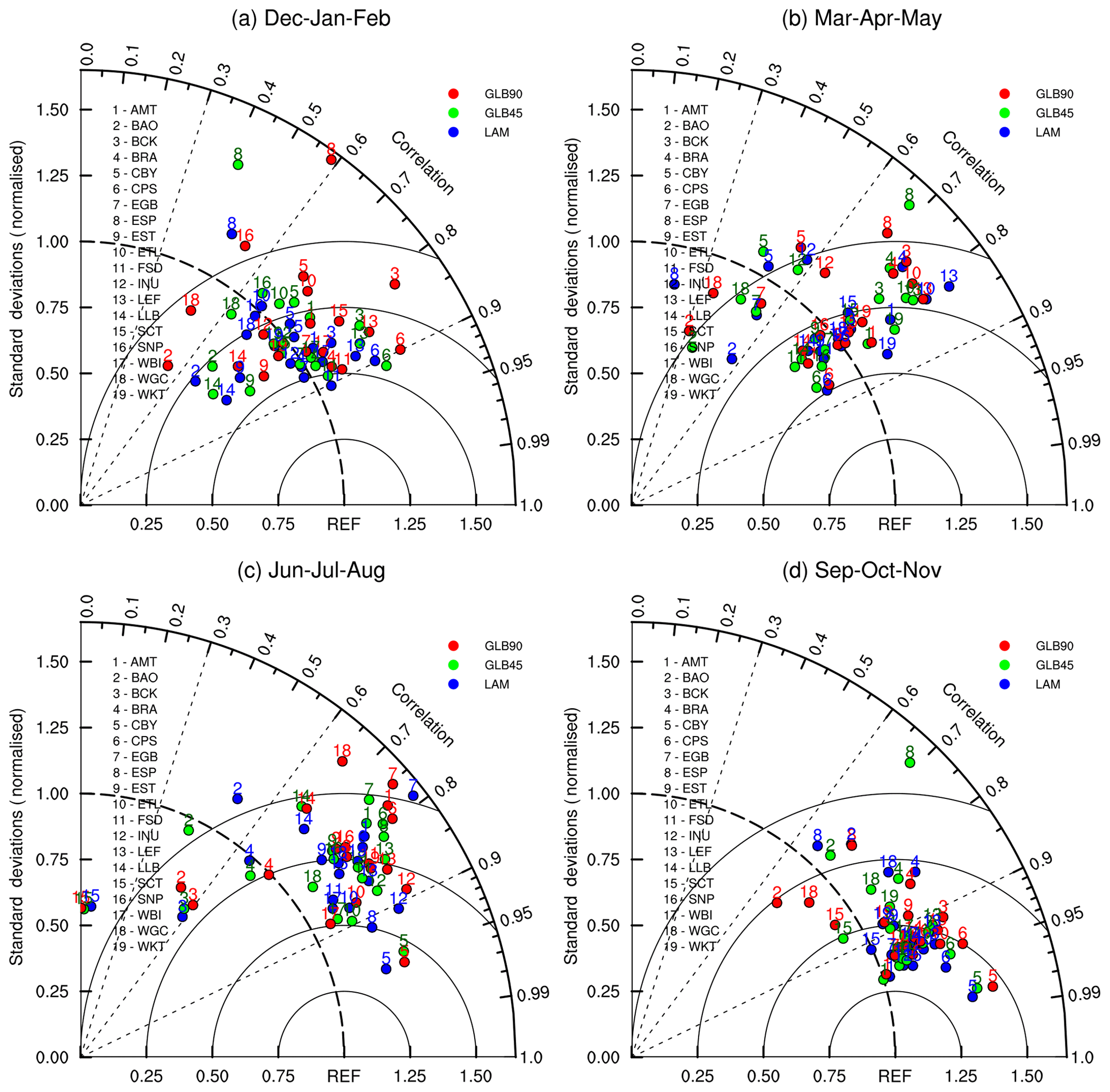
Figure 12Taylor diagram showing correlations and normalised standard deviations between daily afternoon modelled CO₂ concentrations and observed CO₂ concentrations from three models, GLB90 (red), GLB45 (green) and LAM (blue), over (a) January to February and December 2015, (b) March to May 2015, (c) June to August 2015, and (d) September to November 2015.

Download

Thus far, modelled CO₂ concentrations in the afternoon (12:00–16:00 LST) have been analysed. Henceforth, data at all times of the day and night are retained. Figure 13 shows the mean diurnal cycle of modelled and observed CO₂ concentrations for July and December at WGC where the most significant differences among the three experiments are observed. In general, the three experiments simulate similar CO₂ diurnal cycles for other sites (not shown). Data are available for three sampling levels at WGC in 2015. CT2016 is included as well for comparison purposes, but only results at the highest sampling level are shown because only observations at this level were used in the inversion in CT2016. The LAM experiment captures the CO₂ diurnal cycle well, but the GLB90 and GLB45 experiments and CT2016 do not, especially in July (Fig. 13a, c and e). At the sampling level of 483 m, the GLB90 experiment overestimates morning CO₂ concentrations, and CT2016 overestimates nighttime CO₂ concentrations in July, while the GLB45 and LAM experiments capture the diurnal cycle (Fig. 13a) relatively well. This level (483 m) has a comparatively weak diurnal cycle because it is mostly decoupled from the surface at night, and daytime enhancements are significantly diluted relative to lower levels. At lower sampling levels of 91 and 30 m, both the GLB90 and GLB45 experiments overestimate nighttime CO₂ concentrations in July, whereas the LAM experiment captures both day and nighttime CO₂ concentrations well (Fig. 13c and e). This greater sensitivity to model resolution at night was also seen by Agustí-Panareda et al. (2019). WGC is located in a valley between two mountain ranges. The model topographies of GLB90 and GLB45 do not resolve this geography well due to their coarse horizontal resolutions. In contrast, the LAM experiment resolves the actual topography around the WGC site well relative to the two global models. In daytime, CO₂ concentrations are well simulated in the LAM and GLB45 experiments due to the strong vertical mixing (Fig. 13a, c and e). In contrast, accumulated CO₂ in nighttime still remains in the afternoon time in the GLB90 experiment, leading to an overestimation of CO₂ in the afternoon at all sampling levels. In December, the LAM experiment simulates the CO₂ concentration and its standard deviation slightly better at all sampling levels, while the GLB90 and GLB45 experiments underestimate CO₂ concentrations (Fig. 13b, d and f).

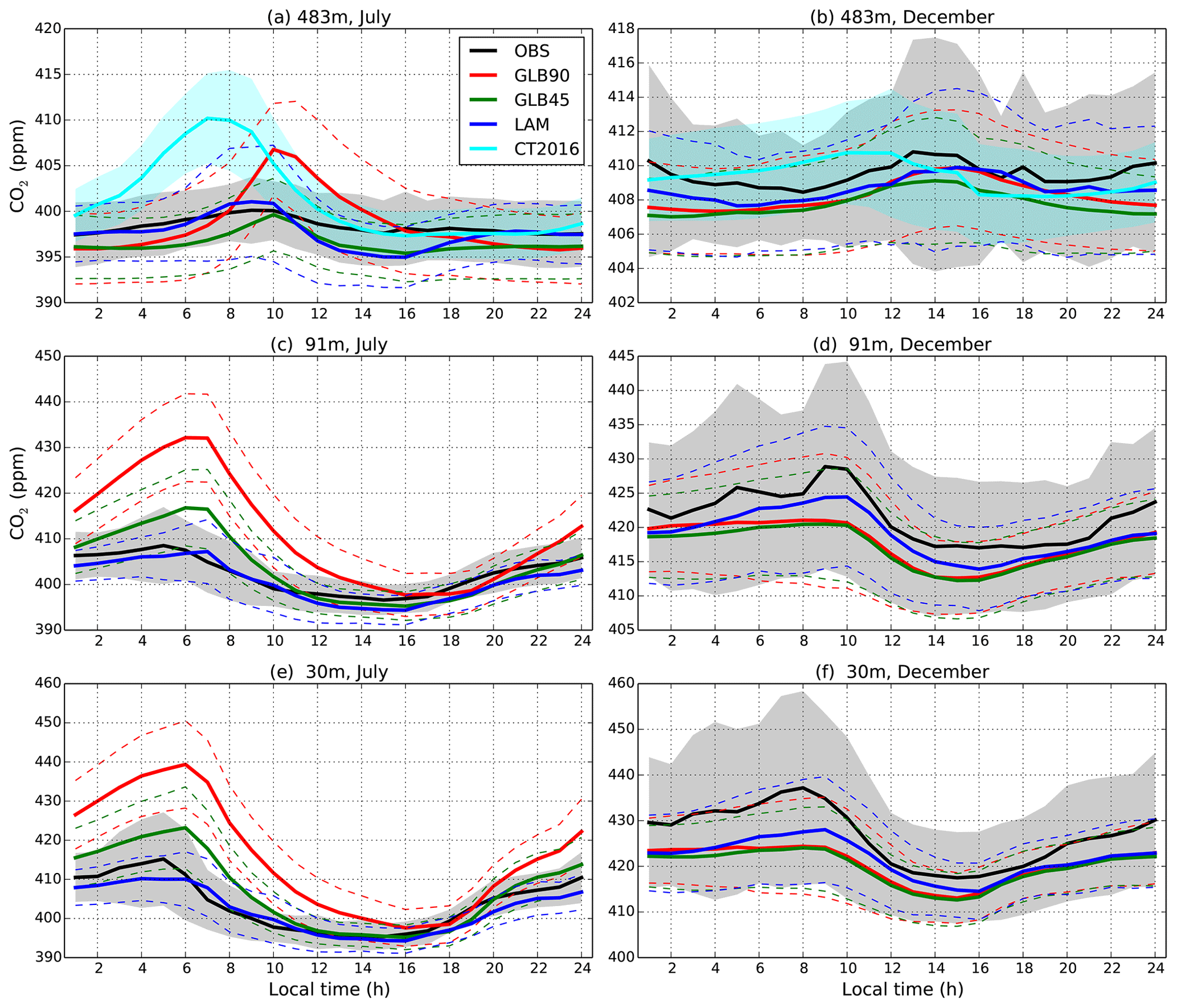
Figure 13Mean diurnal cycle of observed CO₂ concentrations (black) and modelled CO₂ concentrations from the GLB90 (red), GLB45 (green) and LAM (blue) experiments at WGC (Walnut Grove, California) for intake heights of (a) 483 m for July 2015, (b) 483 m for December 2015, (c) 91 m for July 2015, (d) 91 m for December 2015, (e) 30 m for July 2015 and (f) 30 m for December 2015. The grey (cyan) shaded region indicates 1 standard deviation above and below observed (CT2016) CO₂ concentrations, while the dashed lines indicate the same for modelled CO₂ concentrations. Note that CT2016 results are only available at 483 m.

Download

In order to analyse CO₂ time series across various temporal scales beyond the diurnal cycle, the DFT method explained in Sect. 2.5 is applied to hourly CO₂ time series. Figure 14 shows the amplitude of hourly CO₂ concentration time series across different temporal scales from 2 h to 92 d for the period from June to August 2015 at the LEF and WGC sites. Unfortunately, not all sites have hourly observations without missing values for the year 2015. These two sites have hourly data available for 3 months from June to August 2015 without missing values and fortunately reveal different properties. Thus, they were selected to illustrate the impact of increased horizontal resolution on CO₂ simulations on the timescales captured by the models. At LEF, one sampling level, 396 m, satisfies our constraint of no missing data, and at WGC two sampling levels, 483 and 91 m, meet this constraint. At the LEF site, the three experiments capture the signals well across all temporal scales in observed CO₂ time series, including synoptic and diurnal variations (Fig. 14a and b). The topography mismatch of the GLB90 and GLB45 experiments is relatively small at the LEF site. The intake height of measurements at LEF is 396 m above the ground at which laminar flow is more dominant than turbulent flow in nighttime so that the respiration signal from the surface does not reach the free troposphere and synoptic variability is more dominant (Davis et al., 2003; Wang et al., 2007). As a result, the differences in amplitude in the three experiments are less than about 0.8 ppm for all temporal periods (Fig. 14b). At the WGC site, on the other hand, as already shown in Fig. 13, the GLB90 experiment simulates diurnal cycles of CO₂ that are too strong at lower sampling heights in July, which can also be clearly seen in Fig. 14c–f, with the largest overestimation at the lowest sampling level (Fig. 14e and f). However, it is not just the diurnal cycle of CO₂ from June to August that is overestimated in the GLB90 experiment. Periods from sub-diurnal to longer day periods are also overestimated (Fig. 14c–f). Furthermore, while GLB45 performs better than GBL90, it also overestimates the diurnal cycle amplitudes and longer timescales at 483 and 91 m. Hence, the larger mismatch of topography results not only in inaccurate daily timescales but also other scales such as synoptic scales longer than 4 d. A similar result was also found for time periods of 92 to 300 d (Fig. S2). The amplitude of the diurnal cycle can also be computed in model space to illustrate its spatial variability as a function of model resolution (Fig. S3). With the same prescribed fluxes, greater spatial heterogeneity in the diurnal cycle amplitude occurs with increased resolution. However, the validation of these finer spatial scales requires a dense observation network and is not possible at present.

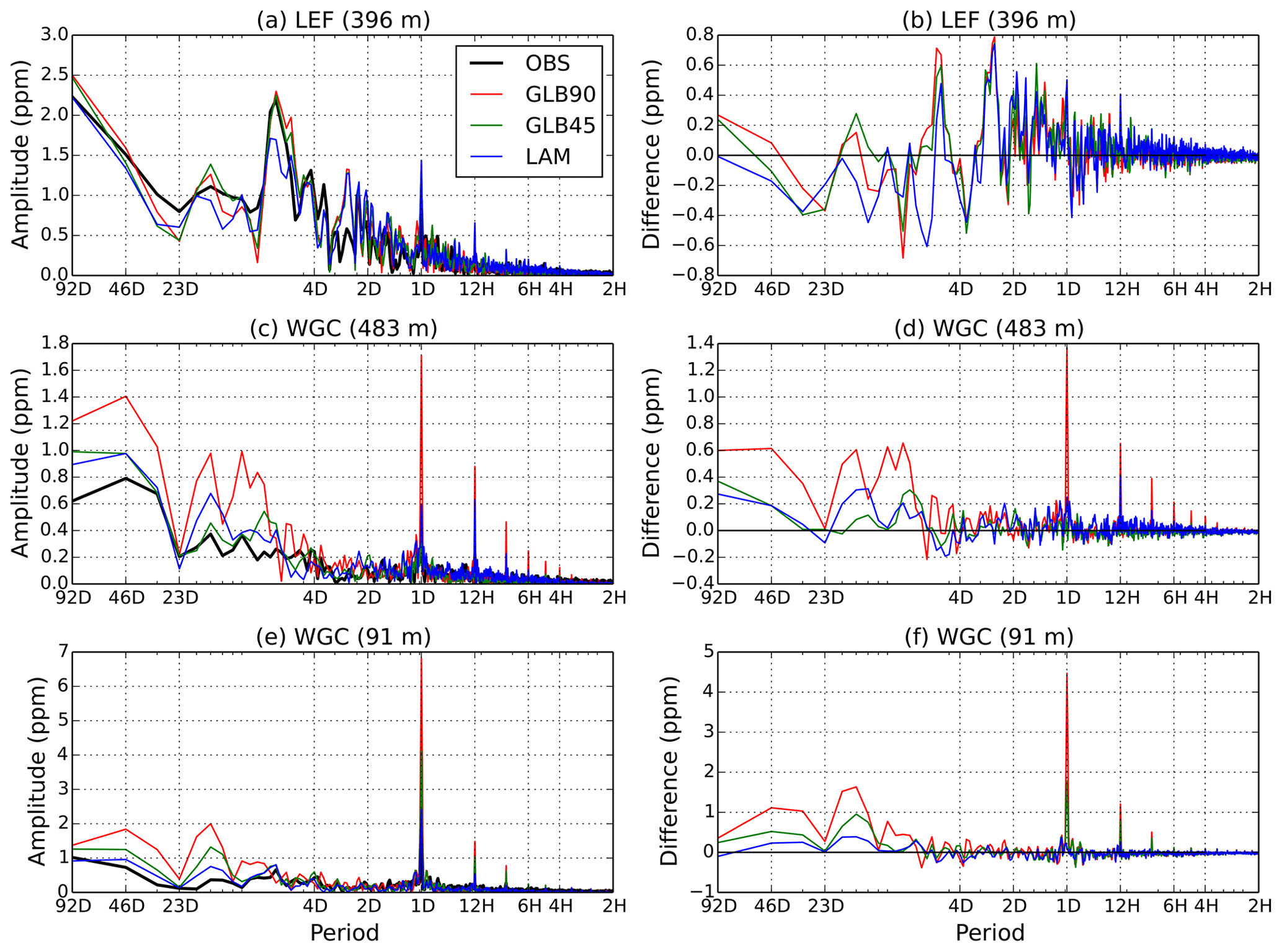
Figure 14The amplitude of hourly time series of observed CO₂ (black) and modelled CO₂ concentrations from the GLB90 (red), GLB45 (green) and LAM (blue) experiments across temporal scales from 2 h to 92 d at (a) LEF (intake height of 396 m) and (b) their differences, (c) WGC (intake height of 483 m) and (d) their differences, and (e) WGC (intake height of 91 m) and (f) their differences.

Download