Implementation of a roughness sublayer parameterization  in the Weather Research and Forecasting model (WRF version 3.7.1) and its evaluation for regional climate simulations

Lee, Junhong; Hong, Jinkyu; Noh, Yign; Jiménez, Pedro A.

doi:https://doi.org/10.5194/gmd-13-521-2020

Articles | Volume 13, issue 2

https://doi.org/10.5194/gmd-13-521-2020

Articles | Volume 13, issue 2

Development and technical paper

11 Feb 2020

Development and technical paper |

| 11 Feb 2020

Implementation of a roughness sublayer parameterization in the Weather Research and Forecasting model (WRF version 3.7.1) and its evaluation for regional climate simulations

Junhong Lee, Jinkyu Hong, Yign Noh, and Pedro A. Jiménez

Abstract

The roughness sublayer (RSL) is one compartment of the surface layer (SL) where turbulence deviates from Monin–Obukhov similarity theory. As the computing power increases, model grid sizes approach the gray zone of turbulence in the energy-containing range and the lowest model layer is located within the RSL. From this perspective, the RSL has an important implication in atmospheric modeling research. However, it has not been explicitly simulated in atmospheric mesoscale models. This study incorporates the RSL model proposed by Harman and Finnigan (2007, 2008) into the Jiménez et al. (2012) SL scheme. A high-resolution simulation performed with the Weather Research and Forecasting model (WRF) illustrates the impacts of the RSL parameterization on the wind, air temperature, and rainfall simulation in the atmospheric boundary layer. As the roughness parameters vary with the atmospheric stability and vegetative phenology in the RSL model, our RSL implementation reproduces the observed surface wind, particularly over tall canopies in the winter season by reducing the root mean square error (RMSE) from 3.1 to 1.8 m s⁻¹. Moreover, the improvement is relevant to air temperature (from 2.74 to 2.67 K of RMSE) and precipitation (from 140 to 135 mm per month of RMSE). Our findings suggest that the RSL must be properly considered both for better weather and climate simulations and for the application of wind energy and atmospheric dispersion.

Download & links

Article (PDF, 8979 KB)

Supplement (3605 KB)

Download & links

Article (8979 KB)
Supplement (3605 KB)
BibTeX
EndNote

How to cite

How to cite.

Dates

Received: 26 Aug 2019 – Discussion started: 02 Oct 2019 – Revised: 21 Dec 2019 – Accepted: 13 Jan 2020 – Published: 11 Feb 2020

1 Introduction

The planetary boundary layer (PBL) is important for the proper simulation of weather, climate, wind energy application, and air pollution. Turbulence plays a critical role in the spatiotemporal variation of the PBL structure through the turbulent exchanges of momentum, energy, and water between the atmosphere and Earth's surface. Because turbulent eddies in the PBL are smaller than the typical grid size in mesoscale and global models, their impacts must be properly parameterized for atmospheric models. The surface layer (SL) occupies the lowest 10 % of the PBL where the shear-driven turbulence is dominant. In the SL, Monin–Obukhov similarity theory (MOST), which is a zero-order turbulence closure, provides the relationships between the vertical distribution of wind and scalars and the corresponding fluxes in a given stability condition (Obukhov, 1946; Monin and Obukhov, 1954). The typical numerical weather prediction (NWP) and climate models are applied for the SL parameterization based on MOST to parameterize the subgrid-scale influences of the turbulent eddies in the PBL (e.g., Sellers et al., 1986, 1996).

The SL has two parts: the inertial sublayer (ISL) and the roughness sublayer (RSL). The ISL is the upper part of the SL, where MOST is valid and vertical variation of the turbulent fluxes is negligible. The RSL is the layer near and within the surface roughness elements (e.g., trees and buildings). The turbulent transport in the RSL has a mixing layer analogy, and the atmospheric flow depends on the roughness element properties (Raupach et al., 1996). Accordingly, the flux–gradient relationships in the RSL deviate from the MOST predictions, and the eddy diffusion coefficients are larger than the values in the ISL (e.g., Shaw et al., 1988; Kaimal and Finnigan, 1994; Brunet and Irvine, 2000; Finnigan, 2000; Hong et al., 2002; Dupont and Patton, 2012; Shapkalijevski et al., 2016; Zhan et al., 2016; Basu and Lacser, 2017).

Traditionally, the RSL has not been explicitly considered in global and mesoscale models because the PBL in the model is coarsely resolved, and the lowest model layer is well above the roughness elements accordingly. As the computing power increases, the grid size of the NWP model decreases and it gets close to the grid size of gray zone for the turbulence. Nevertheless, studies on the impact of a fine vertical resolution have not been relatively performed. From this perspective, the RSL has an important implication in atmospheric modeling research. The lowest model layer is typically approximately 30 m high, and its vertical resolution continues to be better; hence, the models have more than one vertical layer in the RSL, which extends to 2–3 times the canopy height. Furthermore, model outputs are sensitive to the selection of the lowest model level height (Shin et al., 2012), but its relation to the RSL has not yet been clearly investigated. Accordingly, turbulent transport in the RSL must be incorporated particularly in the mesoscale models if the vertical model levels are inside the RSL with an increase in the vertical model resolution.

The RSL function is a popular and simple method of incorporating the effects of the RSL in the observation and model (e.g., Raupach, 1992; Physick and Garratt, 1995; Wenzel et al., 1997; Mölder et al., 1999; Harman and Finnigan, 2007, 2008; de Ridder, 2010; Arnqvist and Bergström, 2015). The RSL function is defined as the observed relationship between the vertical gradient of wind and scalar variables and their corresponding fluxes in the RSL. Accordingly, simple relationships are appropriate for the land surface model in the climate model and for the mesoscale model (Physick and Garratt, 1995; Sellers et al., 1986, 1996). Despite the importance of the RSL, the Weather and Research Forecasting (WRF) model (Skamarock et al., 2008), which is one of the widely used models in the operation and research fields, does not consider the effects of the RSL for the regional weather and climate simulations. Harman and Finnigan (2007, 2008) and Harman (2012) (hereafter, HFs) recently proposed a relatively simpler RSL function that can be used in a wide range of atmospheric models. The RSL function of the HFs is based on a theoretical background and applicable to a wide range of atmospheric stabilities by succinctly satisfying the continuity of the vertical profiles of fluxes, wind, and scalars both at the top of the RSL and at the top of a canopy. The parameterization of HFs has recently been incorporated in a one-dimensional (1-D) PBL model and a land surface model (Harman, 2012; Shapkalijevski et al., 2017; Bonan et al., 2018).

Based on the abovementioned background, this study incorporates the RSL parameterization based on the RSL function of the HFs into the WRF model (version 3.7.1). For this purpose, we reformulate the HFs' RSL parameterization to implement it in the SL parameterization in the WRF model and then discuss the impacts of the RSL parameterization on the regional weather and climate simulations in terms of meteorological conditions near the Earth's surface. To the best of the authors' knowledge, our study is the first extensive attempt to incorporate the RSL parameterization into the WRF model and to validate it for regional climate simulations. Section 2 presents a brief discussion of the RSL parameterization of HFs and the implementation procedures into the WRF model. Section 3 explains the experimental and observational descriptions. Section 4 presents the impacts of the RSL parameterization. Section 5 ends the study with the concluding remarks.

2 RSL theory of the HFs

The roughness sublayer parameterization by HFs is adopted herein along with an explanation of the core of HFs' model, and the relevant details on this parameterization can be found in Harman and Finnigan (2007, 2008) and Harman (2012). Appendix A lists the symbols and variables used in this study in alphabetical order.

We first define the coordinate alignment for its application to the WRF. The revised MM5 SL scheme in the WRF model defines the vertical origin by the conventional zero-plane displacement height (d₀). The same coordinate system is also applied herein. The vertical coordinates z and $\tilde{z}$ in this coordinate system are defined as the distance from d₀ and from the terrain surface, respectively; therefore, their relation is $z = \tilde{z} - d_{0}$ (Fig. 1). Note that a vertical origin in the HFs is at the canopy height (h). MOST says that a variable (C), such as wind speed (u) and temperature (T), has the following logarithmic vertical profile:

\begin{matrix} (1) & \frac{k}{C_{*}} (C (z) - C_{0}) = \ln (\frac{z}{z_{0}}) - ψ_{c} (\frac{z}{L}) + ψ_{c} (\frac{z_{0}}{L}), \end{matrix}

where k is von Kármán constant; C_* is a C scale; C₀ is C at z₀; z₀ is the roughness length; ψ_c is the integrated similarity function of C; and L is the Obukhov length. The C profile based on the RSL function of the HFs is divided into two layers depending on the relative distance between the canopy height and the redefined zero-plane displacement height in the HFs ( $d_{t} = h - d_{0}$ ): the upper-canopy layer (z>d_t), where the influence of additional mixing by the canopy exists, and the lower-canopy layer (z<d_t), where the canopy is the direct source and sink for drag and heat (Fig. 1). The vertical profile in the upper-canopy layer is described as follows:

\begin{matrix} (2) & \begin{aligned} \frac{k}{C_{*}} (C (z) - C_{0}) & = \ln (\frac{z}{z_{0}}) - ψ_{c} (\frac{z}{L}) + ψ_{c} (\frac{z_{0}}{L}) \\ + \int_{z}^{\infty} \frac{ϕ_{c} (1 - {\hat{ϕ}}_{c})}{z^{'}} d z^{'}, \end{aligned} \end{matrix}

where ϕ_c is the similarity function of C, and ${\hat{ϕ}}_{c}$ is an RSL function of C. In the z→∞ limit, ${\hat{ϕ}}_{c}$ is equal to 1 and the wind speed converges to the MOST prediction. The last term on the right-hand side represents the additional mixing caused by the roughness element due to the coherent canopy turbulence and can be replaced by ${\hat{ψ}}_{c}$ , which is an integrated RSL function of C. The vertical profile from the HFs for the RSL deviates from that of MOST because of ${\hat{ψ}}_{c}$ , thereby adjusting the logarithmic profile. The ${\hat{ϕ}}_{c}$ is introduced as follows:

\begin{matrix} (3) & {\hat{ϕ}}_{c} = 1 - c_{1} \exp [- c_{2} \frac{β}{l_{m}} z] . \end{matrix}

c₁ and c₂ are then determined from the continuity of ${\hat{ϕ}}_{c}$ at the canopy top, and the RSL function, ${\hat{ϕ}}_{c}$ , exponentially converges to zero above the RSL. In the lower canopy layer, C has the following exponential form:

\begin{matrix} (4) & C (z) - C_{0} = (C_{h} - C_{0}) \exp (f \frac{z - d_{t}}{2 d_{t}}) . \end{matrix}

The RSL functions vary with atmospheric stability through β:

\begin{matrix} (5) & β = \{\begin{array}{lc} \frac{β_{N}}{ϕ_{m} (z = d_{t})} & \frac{L_{c}}{L} > - 0.15 \\ \frac{k}{2 ϕ_{m} (z = d_{t})} + \frac{\frac{β_{N}}{ϕ_{m} (z = d_{t})} - \frac{k}{2 ϕ_{m} (z = d_{t})}}{1 + 2 {|\frac{L_{c}}{L} + 0.15|}^{1.5}} & \frac{L_{c}}{L} \leq - 0.15 \end{array}, \end{matrix}

where L_c is a canopy penetration depth defined as

\begin{matrix} (6) & L_{c} = {(c_{d} a)}^{- 1} = \frac{4 h}{LAI}, \end{matrix}

where c_d is a drag coefficient at the leaf scale and a is the leaf area density. The parameters d_t and z₀ also depend on the stability because of their dependence on β:

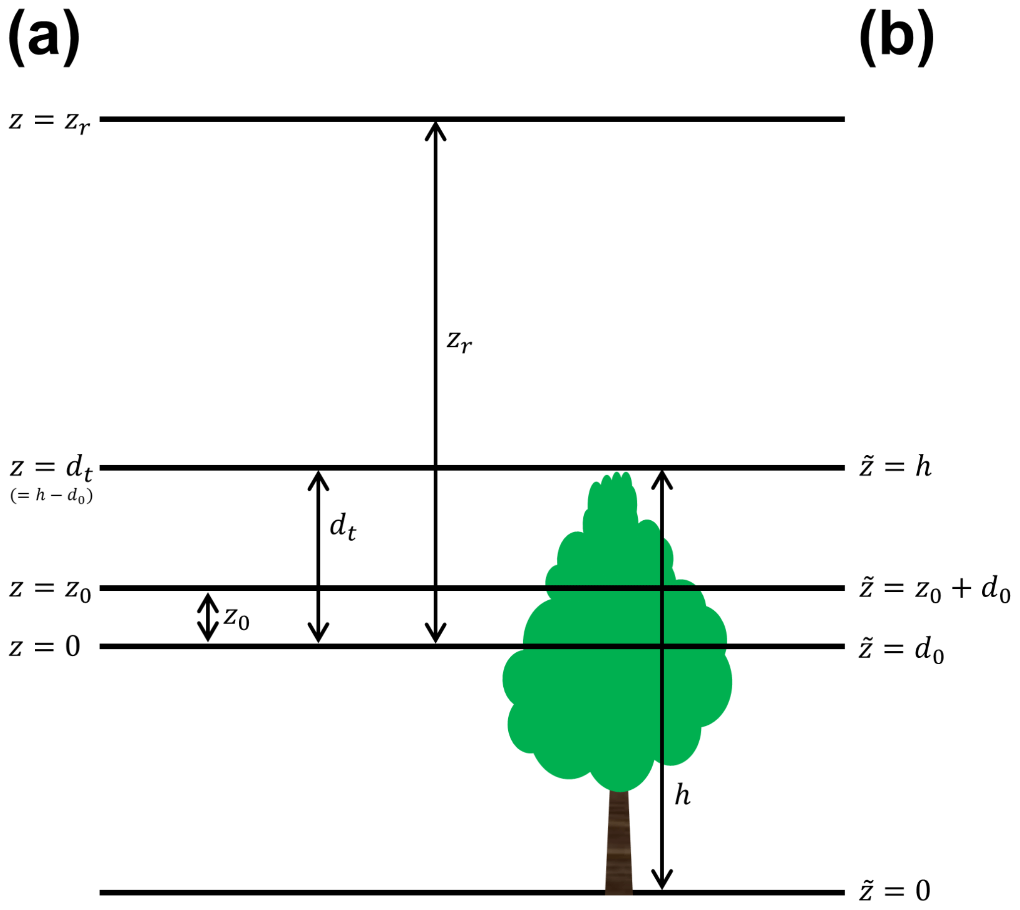
\begin{matrix} (7) & d_{t} = h - d_{0} = \frac{l_{m}}{2 β} = β^{2} L_{c}, \\ (8) & \begin{aligned} z_{0} = & d_{t} \exp [- \frac{k}{β}] \exp [- ψ_{m} (\frac{d_{t}}{L}) + ψ_{m} (\frac{z_{0}}{L})] \\ \exp [\int_{d_{t}}^{\infty} \frac{ϕ_{m} (1 - {\hat{ϕ}}_{m})}{z^{'}} d z^{'}] . \end{aligned} \end{matrix}

https://www.geosci-model-dev.net/13/521/2020/gmd-13-521-2020-f01

Figure 1The schematic diagram to describe the vertical coordinate systems used in this study. (a) The vertical coordinate of the Yonsei University surface layer (YSL) schemes (z) is defined as the distance from the conventional zero-plane displacement height (d₀) and (b) the convectional coordinate ( $\tilde{z}$ ) is defined as the distance from terrain surface. Here, z₀, d_t, h, and z_r are roughness length, the redefined zero-plane displacement height in Harman and Finnigan (2007), canopy height, and the lowest model layer in the conventional coordinate, respectively.

Download

3 Incorporation of the roughness sublayer parameterization into the WRF model

The RSL parameterization of the HFs described above is implemented in the Jiménez et al. (2012) revised MM5 surface layer scheme and Noah land surface model in the WRF (hereafter called the Yonsei University surface layer (YSL) scheme) because of theoretical consistency between the HFs and PBL parameterization. To incorporate the RSL parameterization, it is necessary to modify the SL scheme as follows (Fig. 2): the first step is to compute the bulk Richardson number at the lowest model layer, Bi_b, by the original equation of Jiménez et al. (2012) (Eq. 9 in their study):

\begin{matrix} (9) & B i_{b} = \frac{g}{θ_{a}} \frac{θ_{va} - θ_{vg}}{{[u (z_{r})]}^{2}} z . \end{matrix}

The second step is to iteratively calculate the atmospheric stability (z_r∕L) as follows with an accuracy of 0.01:

\begin{matrix} (10) & \frac{z_{r}}{L} = B i_{b} \frac{{[\ln (\frac{z_{r}}{z_{0}}) - ψ_{m} (\frac{z_{r}}{L}) + ψ_{m} (\frac{z_{0}}{L}) + {\hat{ψ}}_{m}]}^{2}}{[\ln (\frac{ρ c_{p} k u_{*}^{n - 1} z_{r}}{c_{s}} + \frac{z_{r}}{z_{l}}) - ψ_{h} (\frac{z_{r}}{L}) + ψ_{h} (\frac{z_{l}}{L}) + {\hat{ψ}}_{h}]}, \end{matrix}

where $u_{*}^{n - 1}$ is the friction velocity (u_*) at the previous time step. Equation (10) is different from Eq. (23) of Jiménez et al. (2012) by the RSL functions (i.e., ${\hat{ψ}}_{m}$ and ${\hat{ψ}}_{h}$ ). After z_r∕L is determined, the third step is to iteratively update d_t and β using Eqs. (5) and (7) with an accuracy of 0.0001 because they are intercorrelated with each other. Subsequently, z₀ is iteratively achieved with an accuracy of 0.0001 using Eq. (8) at the given z_r∕L, β, and d_t. The u profile is determined using Eqs. (2) and (4). Following Jiménez et al. (2012), the profile of a scalar, such as T, is determined by

\begin{matrix} (11) & \begin{aligned} \frac{k}{C_{*}} (C (z) - C_{0}) & = \ln (\frac{ρ c_{p} k u_{*}^{n - 1} z_{r}}{c_{s}} + \frac{z_{r}}{z_{l}}) - ψ_{c} (\frac{z}{L}) \\ + ψ_{c} (\frac{z_{0}}{L}) + \int_{z}^{\infty} \frac{ϕ_{c} (1 - {\hat{ϕ}}_{c})}{z^{'}} d z^{'}, \end{aligned} \end{matrix}

for the upper-canopy layer. Equation (4) is used for the lower-canopy layer. Finally, u_* is given to

\begin{matrix} (12) & u_{*} = \frac{k u (z_{r})}{[\ln (\frac{z_{r}}{z_{0}}) - ψ_{m} (\frac{z_{r}}{L}) + ψ_{m} (\frac{z_{0}}{L}) + {\hat{ψ}}_{m}]}, \end{matrix}

and the aerodynamic conductance from z=0 to z=z_r(g_a) in the RSL is given to

\begin{matrix} (13) & 1 / g_{a} = \int_{0}^{z_{r}} \frac{d z}{K_{h} (z)} \equiv 1 / g_{a_{1}} + 1 / g_{a_{2}} + 1 / g_{a_{3}} \\ (14) & \begin{aligned} 1 / g_{a_{1}} & \equiv \int_{0}^{z_{l}} \frac{d z}{K_{h} (z)} = \int_{0}^{z_{l}} \frac{d z}{k u_{*} z + \frac{c_{s}}{ρ c_{p}}} \\ = \frac{1}{k u_{*}} \ln [\frac{k u_{*} z_{l}}{c_{s} / ρ c_{p}} + 1] \end{aligned} \\ (15) & 1 / g_{a_{2}} = \int_{z_{l}}^{d_{t}} \frac{d z}{K_{h} (z)} = \frac{S_{c}}{β^{2} u_{h}} [\exp (β \frac{d_{t} - z_{l}}{l_{m}}) - 1], \\ (16) & \begin{aligned} 1 / g_{a_{3}} & = \int_{d_{t}}^{z_{r}} \frac{d z}{K_{h} (z)} = \int_{d_{t}}^{z_{r}} \frac{Φ_{h}}{k u_{*} z} d z = \frac{1}{k u_{*}} [\ln (\frac{z_{r}}{d_{t}}) \\ - ψ_{h} (\frac{z_{r}}{L}) + ψ_{h} (\frac{d_{t}}{L}) + {\hat{ψ}}_{h} (β \frac{z_{r}}{l_{m}}) - {\hat{ψ}}_{h} (β \frac{d_{t}}{l_{m}})] . \end{aligned} \end{matrix}

Computing time increased only 8 % with 61 vertical layers in the YSL scheme despite more iterations in the YSL scheme compared to the revised MM5 SL scheme.

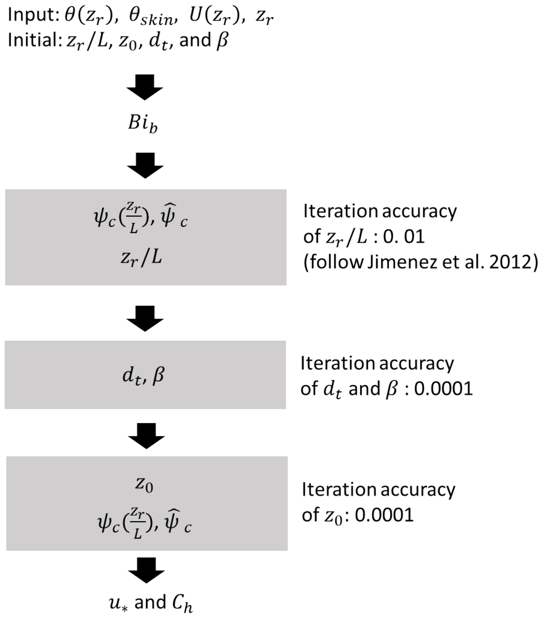
https://www.geosci-model-dev.net/13/521/2020/gmd-13-521-2020-f02

Figure 2Flow diagram of the RSL parameterization. The gray boxes indicate the iteration module.

Download

4 Numerical experimental design

This study evaluated the YSL scheme by making a 1-D offline and real case simulations. The 1-D offline simulations were done to test the YSL scheme performance without feedback with the atmosphere. The 1-D offline simulation consisted of the YSL and the revised MM5 SL schemes coupled with the Noah land surface model (i.e., offCTL and offRSL experiments) (Table 1). In the offline simulations, offCTL and offRSL indicate numerical experiments with and without the RSL parameterization, respectively, and were driven by the idealized forcing data described in Table 1. The real case simulation consisted of two experiments: reproducing 1 month of winter (January 2016) with the revised MM5 SL scheme and the YSL scheme (hereafter referred to as the rCTL and rRSL experiments). The rCTL and the rRSL employed the same physics package, except for the SL scheme and the land surface model (Lee and Hong, 2016 and references therein). One-way nesting was applied herein in a single-nested domain with a Lambert conformal map projection to east Asia (Fig. 3). A 9 km horizontal resolution domain 2 was then embedded in the 27 km resolution domain 1 with 61 vertical layers. The initial and boundary conditions were produced using the National Center for Environmental Prediction Final Analysis data (1^∘ × 1^∘).

Table 1Idealized boundary condition for the one-dimensional offline simulation. Constant z₀ is used only in the CTL experiment.

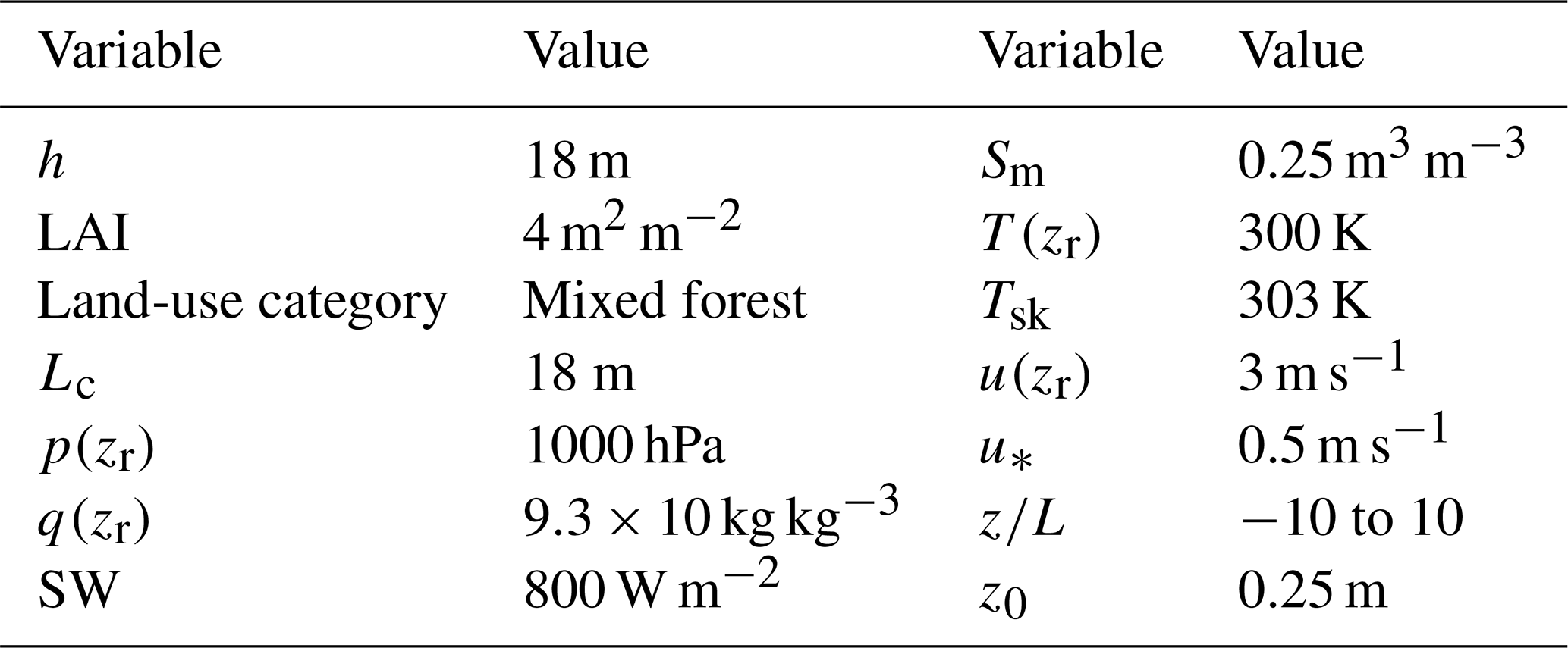
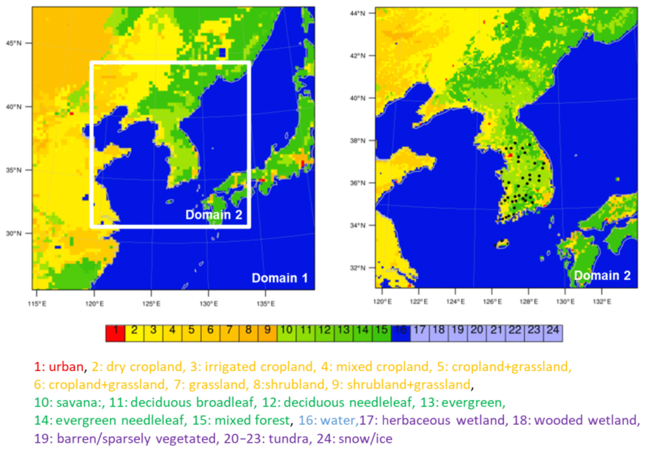
Download Print Version | Download XLSX

https://www.geosci-model-dev.net/13/521/2020/gmd-13-521-2020-f03

Figure 3Domains and land-use category (USGS) of the real case simulation. Black circles denote the automatic synoptic observing system in South Korea used for the model evaluation.

5 Observation data for the model evaluation

The model performance was examined against the surface wind speed, surface temperature and precipitation observed at 46 Automated Synoptic Observing System (ASOS) sites in South Korea (Fig. 3). Quality control of the data includes gap detection, a limit test, and a step test based on the standard of the World Meteorological Administration and Korea Meteorological Administration (KMA) (Zahumenský, 2004; Hong et al., 2019). For the model evaluation of the real case simulation, the three different measures of the correlation coefficients, centered root mean square differences (RSMDs), and standard deviations of the model (σ_m) normalized by that of the observation (σ_o) are together shown in a Taylor diagram (Taylor, 2001). In the Taylor diagram, a point nearer the observation at a reference point (OBS) can be considered to give a better agreement with the observation. We also provide the root mean square error (RMSE) and the mean bias (MB) with the pattern correlation for the rainfall simulation evaluation.

6 Results

6.1 Offline simulations

Figure 4 shows the roughness parameters (i.e., z₀, d_t, and β) as a function of the normalized atmospheric stability (L_c∕L) from the 1-D offline simulation of the YSL scheme (offRSL). The offline YSL simulations reproduced the results of HFs. The roughness parameters varied with the atmospheric stability, L_c∕L, and had peaks at weakly unstable conditions. These dependencies of the roughness parameters on the atmospheric stability are distinct from typical manner of dealing with the roughness parameters as a constant in atmospheric models. The roughness length is indeed constant based on the land cover in all the SL schemes in the WRF.

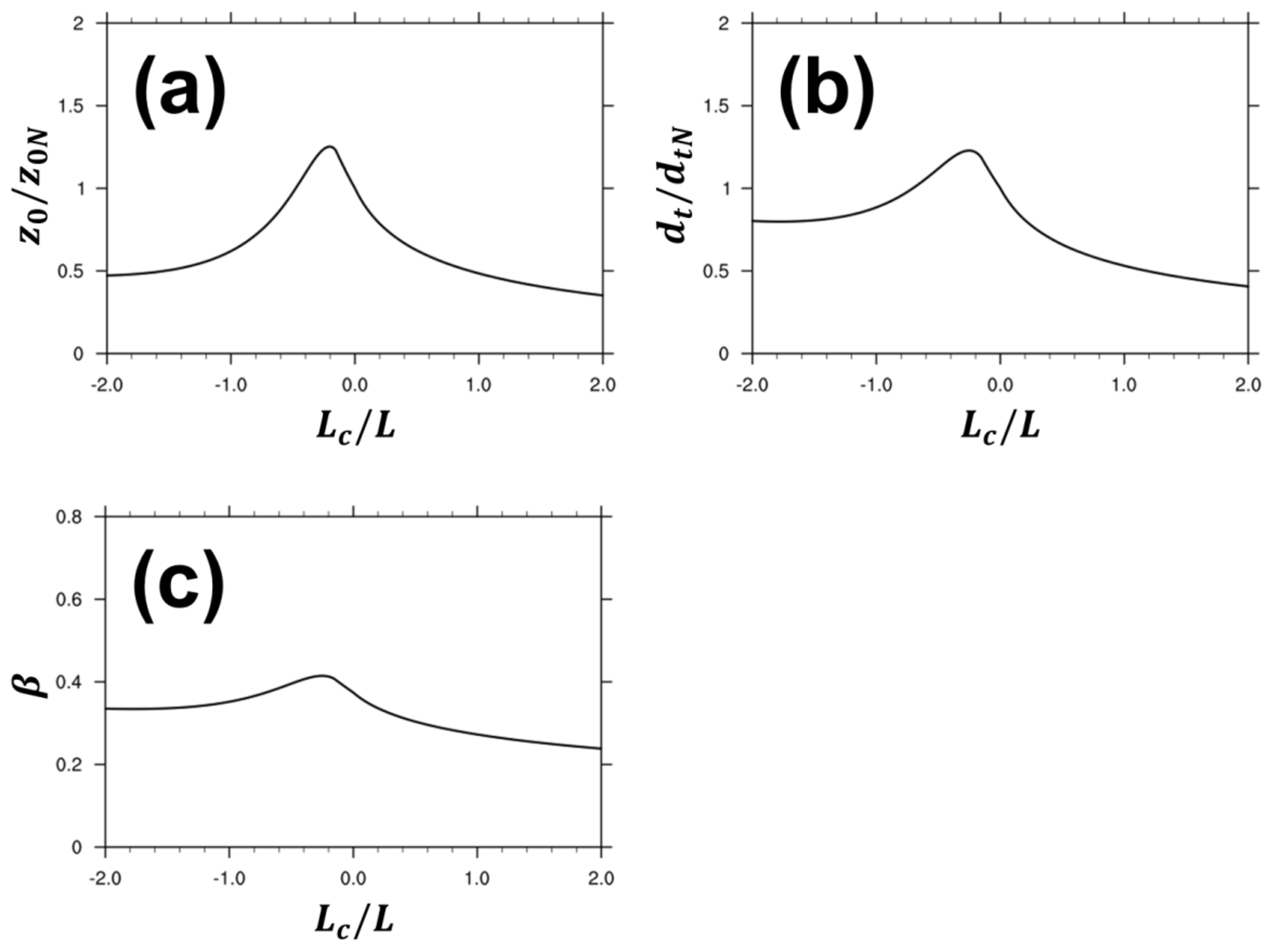
https://www.geosci-model-dev.net/13/521/2020/gmd-13-521-2020-f04

Figure 4Roughness length (a), redefined displacement height (b) and β (c) at a given normalized stability (L_c∕L) from the offRSL simulation with the YSL scheme. Roughness length and redefined displacement height are normalized by their values in a neutral condition (z_0N and d_tN), respectively.

Download

Figure 5 indicates that the impacts of the RSL are also a function of L_c, which is a function of LAI and h (Eq. 6), thus leading to both diurnal and seasonal variation of canopy roughness. Consequently, the roughness parameters showed daily and seasonal variations. Overall, the roughness length in the YSL was larger than that in the revised MM5 SL scheme, particularly in a smaller z∕L (i.e., neutral and unstable conditions) and a larger L_c (i.e., small LAI and/or large h). The roughness length in a stable condition showed relatively smaller changes with z∕L and L_c compared to those in the unstable condition. Our findings suggest that a small LAI in the winter season makes a larger L_c because of the smaller LAI, thereby leading to relatively larger differences of z₀ between the YSL scheme and the default WRF scheme. On the contrary, a similar value of z₀ was observed in summer because of the larger LAI. Note that the revised MM5 SL scheme does not consider d_t and β.

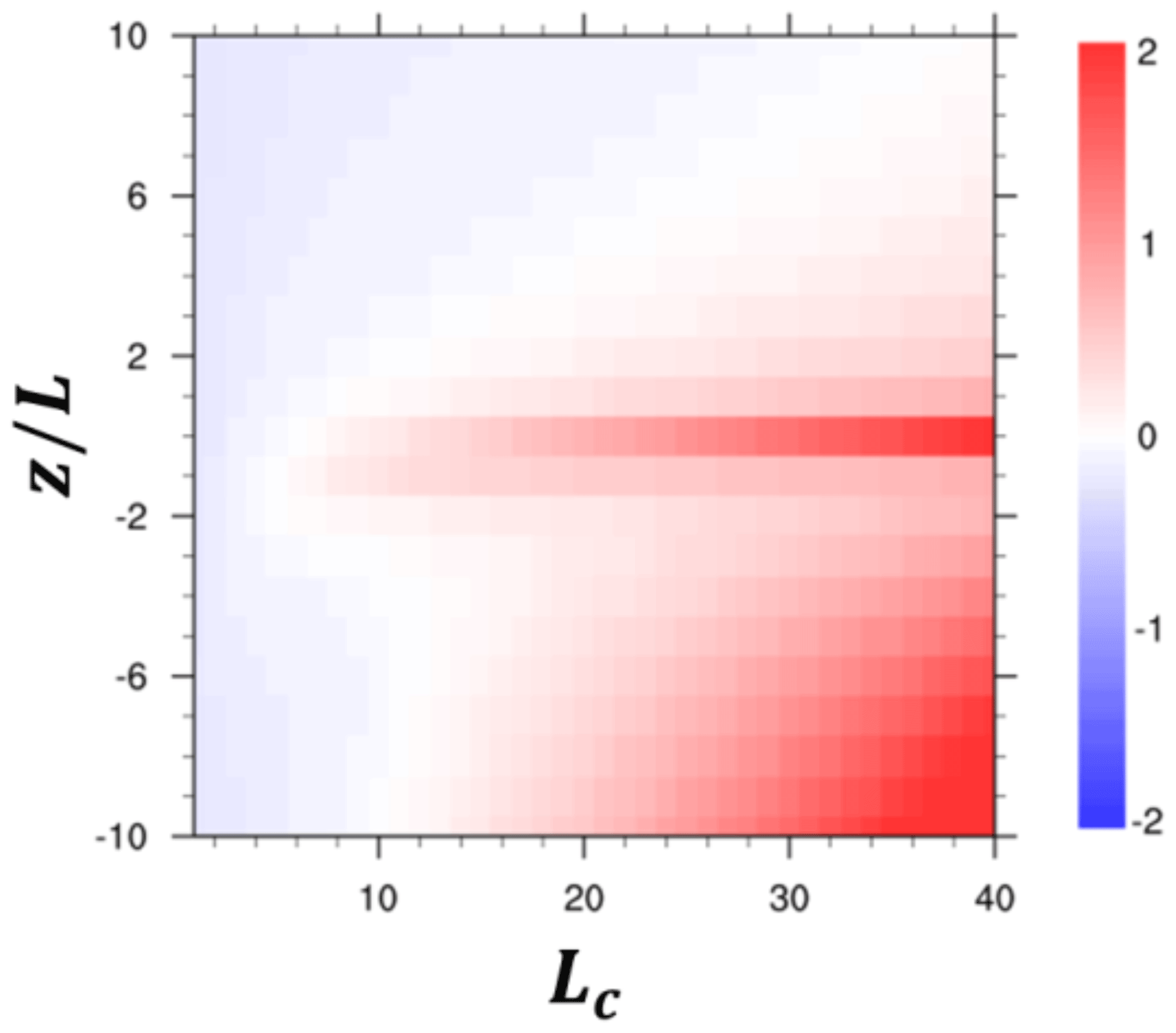
https://www.geosci-model-dev.net/13/521/2020/gmd-13-521-2020-f05

Figure 5Roughness length difference (m) between offCTL and offRSL (offRSL–offCTL) at given atmospheric stability (z∕L) and penetration depth (L_c).

Download

The RSL function, ${\hat{ϕ}}_{c}$ , was introduced to consider the additional mixing caused by the roughness element. Accordingly, ${\hat{ϕ}}_{c}$ should asymptotically converge to the MOST profile (i.e., ${\hat{ϕ}}_{c} \to 1$ ) as z increases with the continuous vertical profiles of the wind and the temperature. The YSL scheme reproduced these properties of ${\hat{ϕ}}_{c}$ and matched with the observed profiles inside canopies: the YSL scheme showed exponential profiles under the canopy top and logarithmic profiles above the canopy top (Fig. 6). The wind speed and the air temperature above the canopy top were smaller than predicted by MOST because ${\hat{ϕ}}_{c} < 1$ in the offRSL experiments. Furthermore, the YSL scheme produced wind and temperature within the canopy (i.e., $\tilde{z} < z_{0} + d_{0}$ ), thereby providing additional useful information on the atmospheric dispersion inside the canopy.

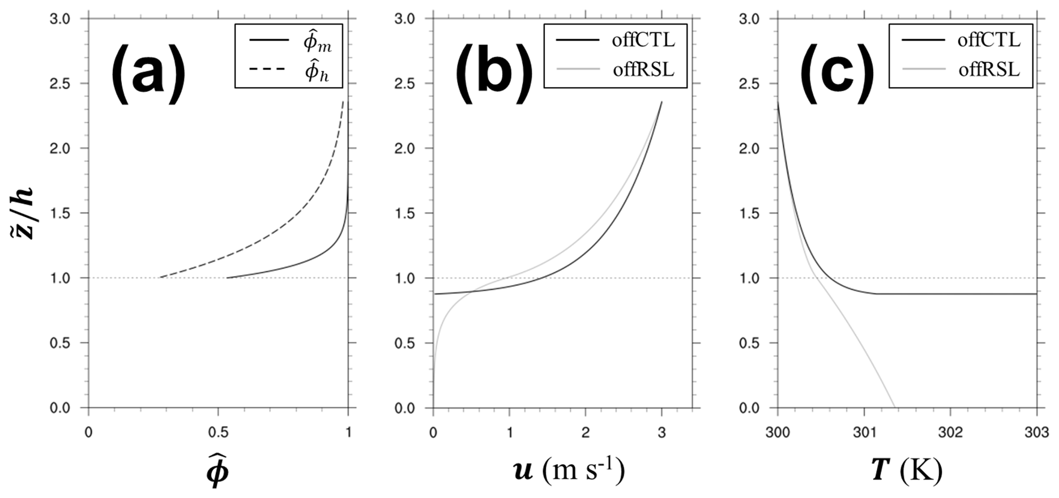
https://www.geosci-model-dev.net/13/521/2020/gmd-13-521-2020-f06

Figure 6(a) Profiles of the RSL function for momentum ( ${\hat{ϕ}}_{m}$ , solid line) and heat ( ${\hat{ϕ}}_{h}$ , dashed line), (b) wind speed (m s⁻¹), and (c) temperature (K) at a neutral condition from offCTL (black) and offRSL (gray). The height of conventional coordinate system ( $\tilde{z}$ ) is normalized by the canopy height (h).

Download

The roughness length changes in the YSL scheme eventually produced changes in the surface energy balance with the atmospheric stability (Fig. 7). In the 1-D offline simulations based on the conditions in Table 1, the YSL scheme produced a larger z₀ in the unstable and near-neutral conditions but a smaller z₀ in $z / L > 3$ compared to the offCTL. The aerodynamic conductance (g_a) in the YSL scheme was larger in all the stability conditions, even in the stable conditions in which the YSL provided a smaller z₀ because the additional term in Eq. (13), $g_{a_{2}}$ , dominated over the other effects in the g_a calculation. Accordingly, H and λE in the YSL scheme were larger than those in the revised MM5 SL scheme. Our finding implies stronger fluxes from the YSL scheme when the gradient of quantity is the same. However, the impact of the increased g_a was asymmetrical in H and λE depending on the soil moisture content. In this case simulation, an increase in λE was dominant because the wet condition made more partitioning of the available energy into the latent heat flux first in the model. However, in the dry condition (i.e., less soil water content), the YSL produced a larger H without a substantial increase of λE (Fig. S1 in the Supplement). A significant increase in λE was found along with a decrease in H in the strong unstable conditions (Fig. 7) because of the wet soil moisture of 0.25 m³ m⁻³ in the offRSL simulation in Table 1. The slight increase in the net radiation was mainly associated with the reduced outgoing longwave radiation caused by the smaller surface temperature in the offRSL.

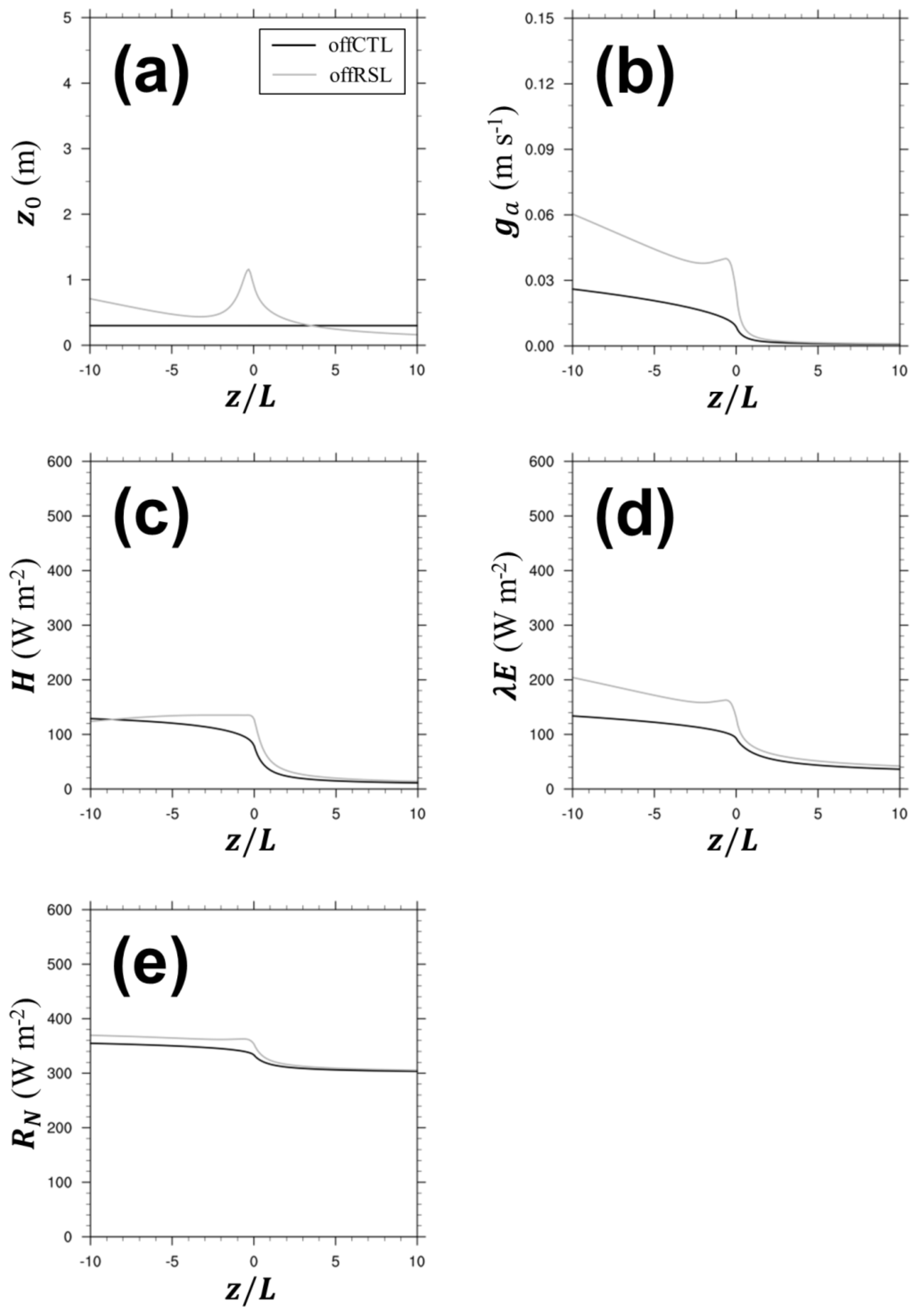
https://www.geosci-model-dev.net/13/521/2020/gmd-13-521-2020-f07

Figure 7(a) Roughness length (m), (b) aerodynamic conductance (m s⁻¹), (c) sensible heat flux (W m⁻²), (d) latent heat flux (W m⁻²), and (e) net radiation (W m⁻²) at a given atmospheric stability (z∕L). The black lines denote offCTL, while the gray lines denote offRSL.

Download

6.2 Real case simulations

Figure 8 shows the real case simulation of the roughness length, 10 m wind speed (u₁₀), and 2 m air temperature (T₂). We discuss herein the real cases in the winter season because of stronger effect of the roughness sublayer. The results for the summer season can be found in the Supplement. The roughness length in the rCTL experiment was prescribed from the vegetation data table (i.e., VEGPARM table in the WRF model) and modified by the vegetation fraction (Fig. 8a).

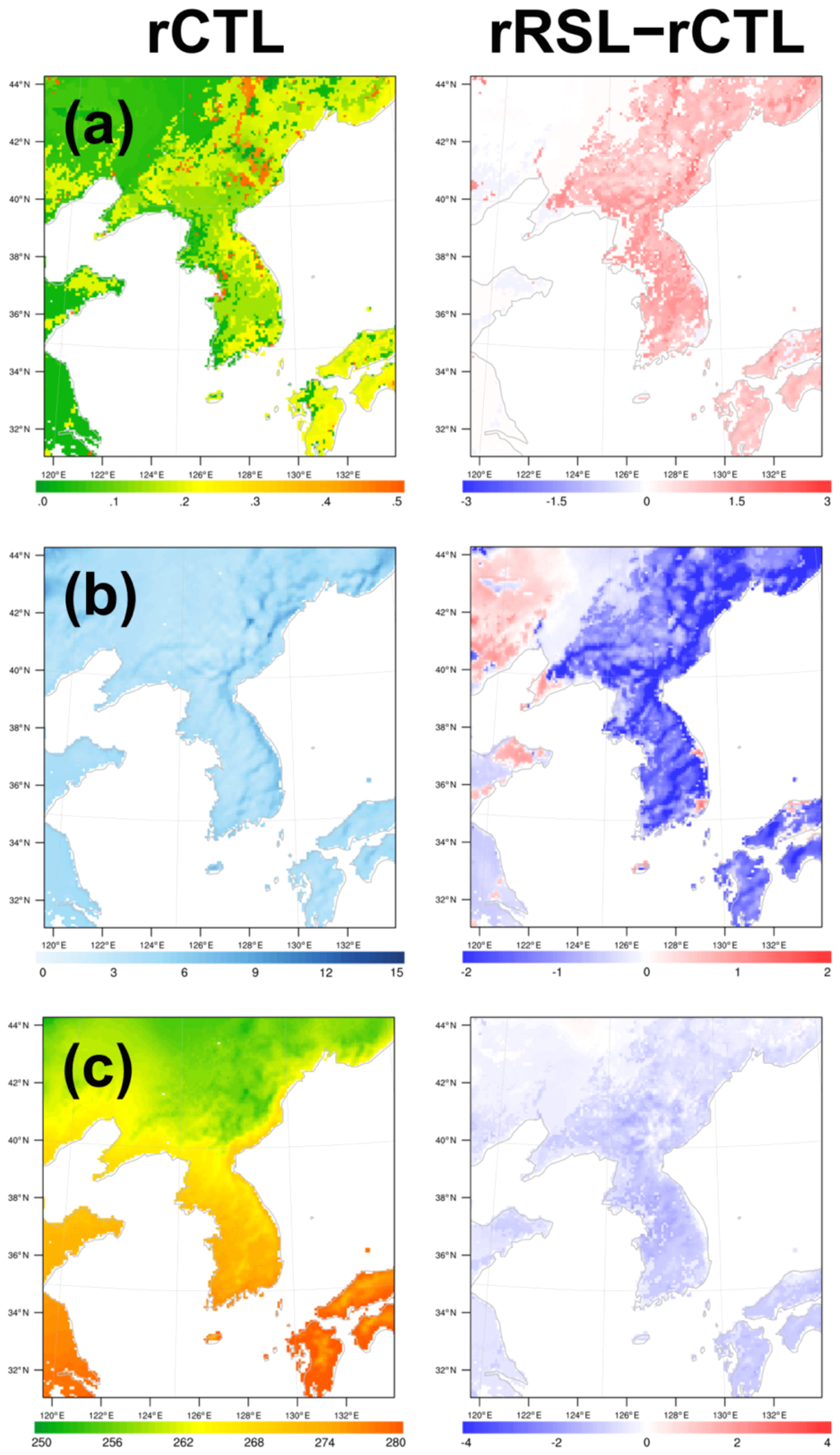
https://www.geosci-model-dev.net/13/521/2020/gmd-13-521-2020-f08

Figure 8(a) Roughness length (m), (b) 10 m wind speed (m s⁻¹), and (c) daytime 2 m temperature (K) of the (left) rCTL experiment and (right) the difference (rRSL–rCTL). The results are averaged over a period of 1 month and masked out over the ocean.

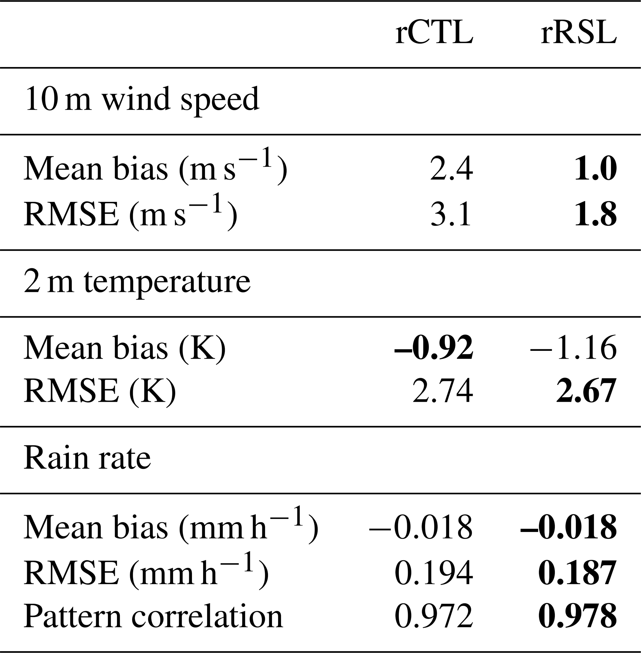
Overall, the YSL scheme (rRSL experiment) produced 0.2–2.0 m larger z₀ than the default values in the rCTL experiment over the tall canopies, where L_c was large. In contrast, the YSL scheme produced a similar or even slightly smaller z₀ over the short canopies compared to the rCTL experiment. Importantly, the changes of z₀ made direct impacts on the momentum fluxes and thus surface wind speed (Fig. 8b). The typical u₁₀ in the rCTL was larger than approximately 3 m s⁻¹, and a much stronger wind (>6 m s⁻¹) was observed along the mountains, making a positive bias against the observation. Overall, the YSL scheme reproduced the better observed diurnal variation by reducing the positive bias of the wind speed (Table 2, Fig. 9). Over the tall forest canopies, u₁₀ in the rRSL was reduced by approximately 30 %; however, the region of the increased wind speed corresponded to the short canopies, where the roughness length increased (Fig. 8a and b). The YSL scheme particularly provided a better RMSD and correlation coefficient but less diurnal variability of wind speed because of a relatively larger reduction of the daytime wind speed (Fig. 9). MB and RMSE decreased from 2.4 to 1.0 m ⁻¹ and from 3.1 and 1.8 m s⁻¹. The Taylor diagram shows that the overall performance of the YSL scheme is better than the default WRF simulation at all the 46 sites. In the Taylor diagram, the statistics moved toward the observation, except for one site, indicating an overall improvement of 2 m air temperature in the YSL scheme; however, the impact of the RSL was not as large as the wind speed (Table 2, Fig. 10).

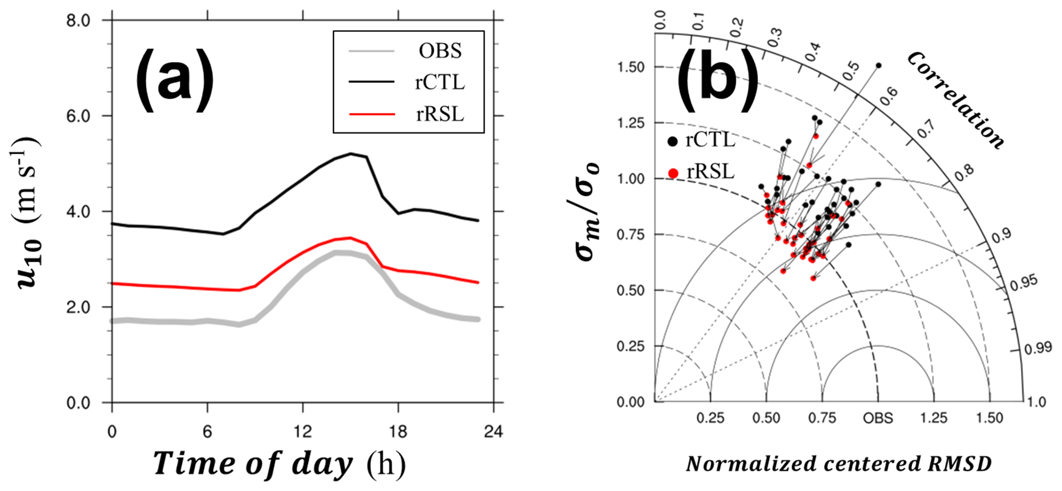
https://www.geosci-model-dev.net/13/521/2020/gmd-13-521-2020-f09

Figure 9(a) A 1-month mean diurnal variation of 10 m wind speed and (b) the Taylor diagram showing the correlation coefficient, normalized centered root mean square differences (RMSDs), and standard deviations of the models (σ_m) normalized by that of observation (σ_o) from observation (gray), rCTL experiment (black), and rRSL experiment (red). The vectors indicate the changes of the statistics from rCTL to rRSL. The arrows indicate those from rCTL to rRSL. Every vector shows the movement toward the observation, thereby suggesting the model improvement.

Download

https://www.geosci-model-dev.net/13/521/2020/gmd-13-521-2020-f10

Figure 10Same as in Fig. 9 but for the 2 m temperature.

Download

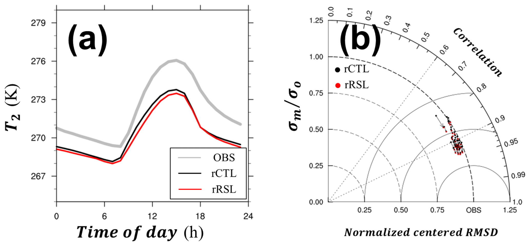
Table 2Statistics of the 10 m wind speed, 2 m temperature, and rain rate. The top statistics are presented in bold.

Download Print Version | Download XLSX

Similar to the increases of the aerodynamic conductance in the offline simulations, the YSL scheme in the real case simulation (i.e., the rRSL simulation) simulated a larger g_a, particularly in the forest canopies and mountain regions (Fig. 11a). This larger g_a in the YSL scheme led to the increases of the latent heat fluxes by approximately 20 W m⁻², with an eventual reduction of the soil water content (Fig. 12a). The sensible heat fluxes in the rCTL experiments were generally approximately 80 W m⁻², except over the snow-covered region where H was approximately 40 W m⁻². As described in the offline simulation, the changing sign of H in the rRSL depended on the soil moisture content because evapotranspiration is limited in dry soils at given available energy (Figs. 11b and 12b). Consequently, the available energy ( $= H + λ E$ ) increased in the YSL scheme, and a larger λE in the rRSL led to a cooler temperature than that in the rCTL experiment (Fig. 8c).

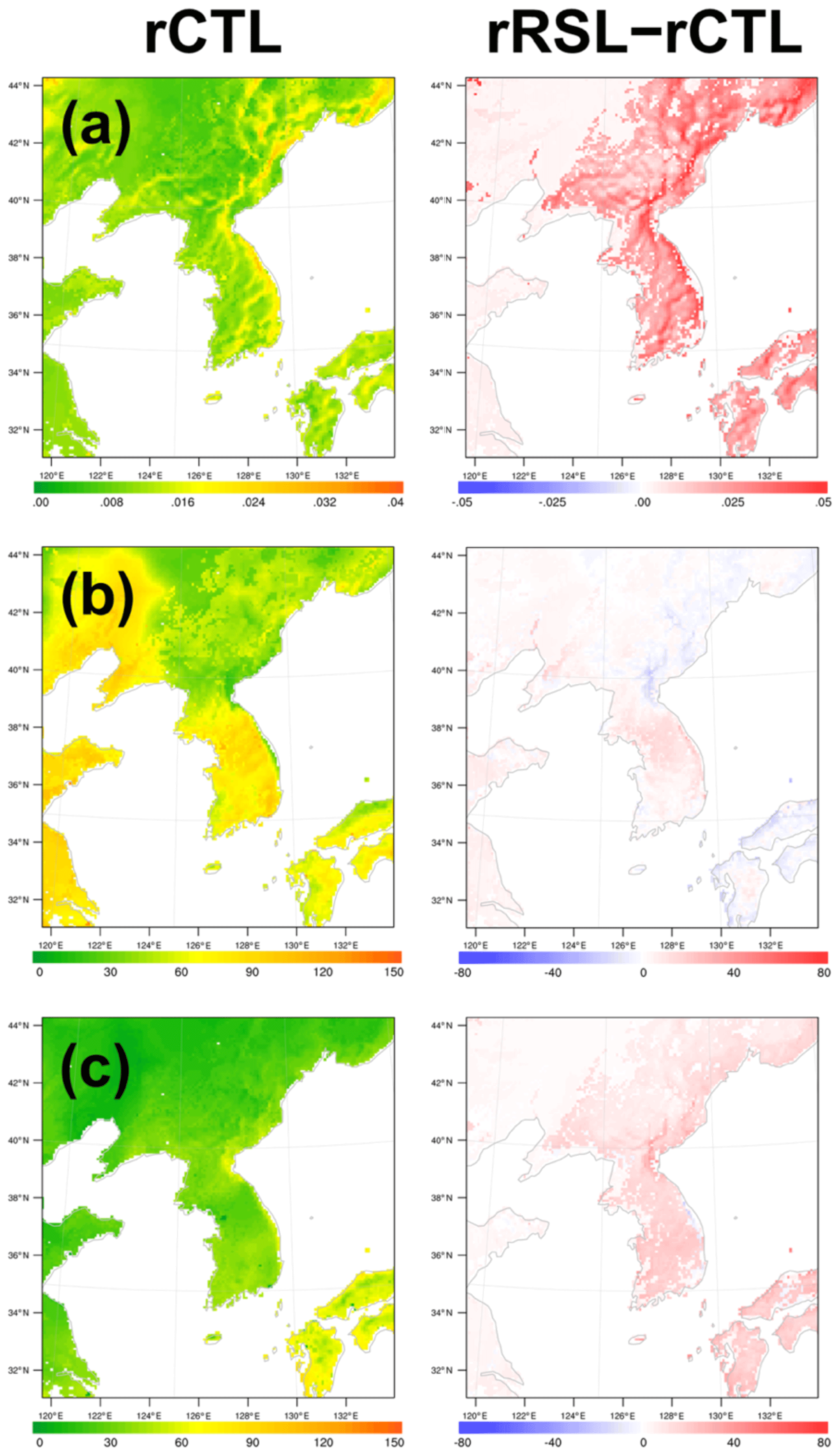
https://www.geosci-model-dev.net/13/521/2020/gmd-13-521-2020-f11

Figure 11(a) Aerodynamic conductance (m s⁻¹), (b) daytime sensible heat flux (W m⁻²), and (c) daytime latent heat flux (W m⁻²) of the (left) rCTL experiment and (right) the difference (rRSL–rCTL). The results are averaged over a period of 1 month and masked out over the ocean.

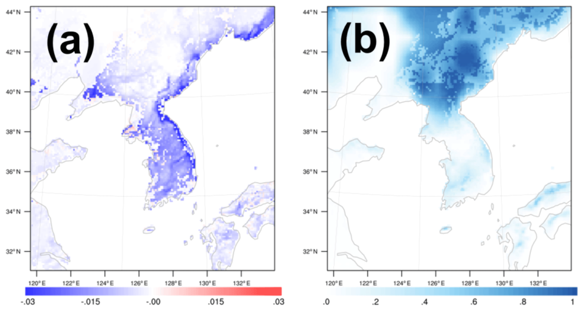
https://www.geosci-model-dev.net/13/521/2020/gmd-13-521-2020-f12

Figure 12(a) Difference of the soil moisture (m³ m⁻³) (rRSL–rCTL) and (b) snow cover (%) of rCTL. The results are averaged over a period of 1 month and masked out over the ocean.

During the winter simulation period, precipitation was observed over an extensive area in the domain, and snow was dominant over the northeastern side of the domain (Figs. 12b and 13). The overall total precipitation in the YSL scheme increased, and the skill score indicated a better simulation of the total amount of precipitation (Table 2, Fig. 13). The pattern correlation of precipitation also increased from 0.972 to 0.978 in the YSL scheme based on 656 rain gauge stations, indicating a better match of the precipitation bands. Despite the increase in λE, precipitation decreased in several regions (Figs. 11b and 13b). The differences were not significant in the summer season, and the skill scores in the YSL scheme were similar to the default WRF simulation because our implemented RSL parameterization started to converge to the default WRF in a smaller L_c (i.e., larger LAI and/or smaller h) and strong synoptic influences by the summer heavy rainy period (Table S1 in the Supplement, Figs. S2–S6).

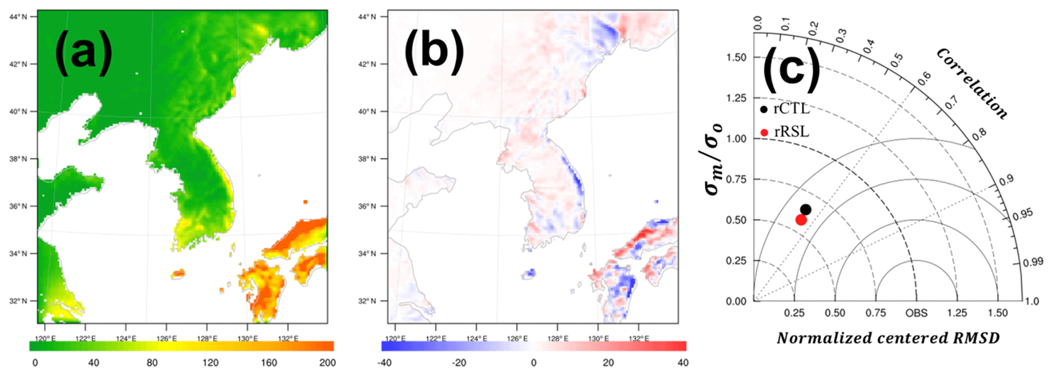
https://www.geosci-model-dev.net/13/521/2020/gmd-13-521-2020-f13

Figure 13(a) The 1-month accumulated precipitation of the rCTL experiment (mm) and (b) difference (rRSL–rCTL). (c) Taylor diagram showing the correlation coefficient, normalized centered RMSD, and the standard deviations of models (σ_m) normalized by that of the observation (σ_o) and from the rain rate (mm h⁻¹) of the rCTL experiment (black) and the rRSL experiment (red) during 1 month at 656 rain gauges.

7 Summary and concluding remarks

Turbulent fluxes regulate the planetary boundary layer; thus, they are a crucial process for weather, climate, and air pollution simulations. Most of the NWP and climate models are commonly applied for MOST to compute the turbulent fluxes near the Earth's surface. MOST can be only applicable in the inertial layer and turbulence deviates from MOST in the roughness sublayer. Importantly, the roughness sublayer, the important compartment of the SL, has not been properly parameterized in the model. Increasing the computing power enables us to use more vertical layers in the atmospheric models. Accordingly, the RSL must be incorporated into the model properly to simulate the atmospheric processes in the gray zone. This study proposed the YSL scheme, which incorporated the RSL into the WRF model, based on the RSL model proposed by Harman and Finnigan (2007, 2008) and Harman (2012). We also investigated the impacts of the RSL parameterization on the weather and climate simulations. For these purposes, we designed a series of offline simulations with an idealized boundary condition and real case simulations to evaluate the performance of the YSL scheme against the observation data.

The 1-D offline simulation revealed that the YSL scheme successfully reproduced the features reported in various canopies. The RSL function, ${\hat{ϕ}}_{c}$ , asymptotically increased to 1, and the vertical gradients of the wind speed and the temperature decreased in the RSL as z increased, thereby converging to the MOST prediction. Notably, unlike the typical assignment of the roughness parameters (i.e., z₀, d_t, and β) as a constant, the roughness parameters are functions of the atmospheric stability (z∕L) and L_c. The roughness parameters had a maximum in the weakly unstable condition and in larger L_c (i.e., large h or small LAI). In most conditions, the YSL scheme provided a larger roughness length, thereby producing a wind speed slower than that of the revised MM5 SL scheme. The YSL scheme simulated a colder surface temperature in the unstable conditions.

Meanwhile, the real case simulation showed that the RSL-incorporated WRF produced a larger z₀ than the default WRF. This increase in z₀ and its change with atmospheric stability eventually made substantial impacts on wind, and temperature near the surface, momentum transfer, surface energy balance, and precipitation. First, an increase of z₀ produced larger momentum fluxes and a smaller 10 m wind speed when the YSL scheme was applied, leading to the mitigation of positive bias in the wind speed in the revised MM5 SL scheme. The larger z₀ also made increases in the available energy. This increased available energy is related to the surface cooling caused by the increases in the latent heat fluxes in the wet surface conditions when the RSL parameterization is applied. As a result, these changes in the climate near the surface and the surface energy balance resulted in more precipitation, thereby giving a better simulation of the amount of precipitation and its spatial pattern.

Our results indicate that the RSL parameterization can be a promising option for resolving the typical overestimation of the surface wind speed of the WRF model, particularly in the tall vegetation and low LAI, with slight increase of computing time (e.g., Hu et al., 2010, 2013; Shimada and Ohsawa, 2011; Shimada et al., 2011; Wyszogrodzki et al., 2013; Lee and Hong, 2016). The improvement caused by the RSL parameterization is useful in air quality modeling and wind energy estimation by better weather and climate in the planetary boundary layer. A further study is necessary to evaluate the characteristics of the YSL scheme in various cases particularly at gray-zone resolutions.

Appendix A: List of symbols and definitions

Symbols	Definitions
a	Leaf area density
Bi_b	Bulk Richardson number, at the lowest model layer
c_d	Drag coefficient at the leaf level
c_p	Specific heat for air
c_s	Effective heat transfer coefficient for nonturbulent processes (Carlson and Boland, 1978; Jiménez et al., 2012)
C	Variable at z, such as u and T
C₀	C at z=z₀
C_h	C at h
C_*	Scale of C
d₀	Conventionally defined zero-plane displacement height
d_t	Redefined zero-plane displacement height in Harman and Finnigan (2007)
f	Parameter related the depth scale of the scalar profile ( $\equiv \frac{1}{2} (\sqrt{1 + 4 r_{c} S_{c}} - 1))$
g	Gravitational acceleration
g_a	Aerodynamic conductance
h	Canopy height
k	von Kármán constant
l_m	Mixing length for momentum
L	Obukhov length
L_c	Canopy penetration depth ( $\equiv (c_{d} a)^{- 1} = \frac{4 h}{LAI}$ )
LAI	Leaf area index
p	Pressure at z
q	Water vapor mixing ratio at z
r_c	Canopy Stanton number
SW	Downward shortwave radiation
S_c	Turbulent Schmidt number at canopy top
S_m	Soil moisture
T	Air temperature at z
T₂	Air temperature at 2 m
T_sk	Skin temperature
u	Wind speed at z
u₁₀	Wind speed at 10 m
u_h	Wind speed at h
u_*	Friction velocity
$u_{*}^{n - 1}$	Previous time step value of u_*
z	Height from d₀
$\tilde{z}$	Height from terrain surface
z₀	Roughness length
z_l	Viscous sublayer depth = 0.001 (Carlson and Boland, 1978; Jiménez et al., 2012)
z_r	Height of the lowest model layer
z_r∕L	Atmospheric stability
β	$u_{*} / u_{h}$
β_N	β at neutral condition (=0.374)
θ_a	Potential temperature of the air at z_r
θ_va	Virtual potential temperature of the air at z_r
θ_vg	Virtual potential temperature of the air at ground
ρ	Density of air
ϕ_C	Similarity function of C
${\hat{ϕ}}_{C}$	RSL function of C
ψ_C	Integrated similarity function of C
ψ_h	Integrated similarity function of heat
ψ_m	Integrated similarity function of momentum
${\hat{ψ}}_{C}$	Integrated RSL function of C
${\hat{ψ}}_{h}$	Integrated RSL function of heat
${\hat{ψ}}_{m}$	Integrated RSL function of momentum

Code and data availability

The source code of the Weather Research and Forecasting model (WRF) (Skamarock et al., 2008) is available at http://www2.mmm.ucar.edu/wrf/users/downloads.html (last access: 4 February 2020). The source code of the YSL scheme and the modeling output presented in this study are available at Zenodo (https://doi.org/10.5281/zenodo.3555537) (last access: 4 February 2020). The National Centers for Environmental Prediction Final Analysis data that were used as initial and boundary conditions are available at https://rda.ucar.edu/datasets/ds083.2 (last access: 4 February 2020) (National Centers for Environmental Prediction, National Weather Service, NOAA, US Department of Commerce, 2000). The observation data used for the model evaluation can be downloaded at the Korea Meteorological Administration data portal (https://data.kma.go.kr/data/grnd/selectAsosRltmList.do?pgmNo=36) (last access: 4 February 2010) or are available upon request to the corresponding author (jhong@yonsei.ac.kr/http://eapl.yonsei.ac.kr, last access: 10 February 2020).

Supplement

The supplement related to this article is available online at: https://doi.org/10.5194/gmd-13-521-2020-supplement.

Author contributions

JL and JH contributed to the code development for the YSL scheme, data analysis, and manuscript preparation. YN and PAJ contributed to the writing and editing of the paper and data analysis.

Competing interests

The authors declare that they have no conflict of interest.

Acknowledgements

Our thanks go to the editor and anonymous reviewers for their constructive comments.

Financial support

This research has been supported by the National Research Foundation of Korea grant funded by the South Korean government (MSIT) (grant no. NRF-2018R1A5A1024958), the Korea Meteorological Administration Research and Development Program (grant no. KMI2018-03512), and the Korea Polar Research Institute (grant no. PN20081).

Review statement

This paper was edited by Jatin Kala and reviewed by two anonymous referees.

References

Arnqvist, J. and Bergström, H.: Flux-profile relation with roughness sublayer correction, Q. J. Roy. Meteorol. Soc., 141, 1191–1197, 2015.

Basu, S. and Lacser, A.: A Cautionary Note on the Use of Monin–Obukhov Similarity Theory in Very High-Resolution Large-Eddy Simulations, Bound.-Lay. Meteorol., 163, 351–355, 2017.

Bonan, G. B., Patton, E. G., Harman, I. N., Oleson, K. W., Finnigan, J. J., Lu, Y., and Burakowski, E. A.: Modeling canopy-induced turbulence in the Earth system: a unified parameterization of turbulent exchange within plant canopies and the roughness sublayer (CLM-ml v0), Geosci. Model Dev., 11, 1467–1496, https://doi.org/10.5194/gmd-11-1467-2018, 2018.

Brunet, Y. and Irvine, M. R.: The control of coherent eddies in vegetation canopies: streamwise structure spacing, canopy shear scale and atmospheric stability, Bound.-Lay. Meteorol., 94, 139–163, 2000.

Carlson, T. N. and Boland, F. E.: Analysis of urban-rural canopy using a surface heat flux/temperature model, Bound.-Lay. Meteorol., 17, 998–1013, 1978.

de Ridder, K.: Bulk transfer relations for the roughness sublayer, Bound.-Lay. Meteorol., 134, 257–267, 2010.

Dupont, S. and Patton, E. G.: Momentum and scalar transport within a vegetation canopy following atmospheric stability and seasonal canopy changes: the CHATS experiment, Atmos. Chem. Phys., 12, 5913–5935, https://doi.org/10.5194/acp-12-5913-2012, 2012.

Finnigan, J. J.: Turbulence in plant canopies, Annu. Rev. Fluid Mech., 32, 519–571, 2000.

Harman, I. N.: The role of roughness sublayer dynamics within surface exchange schemes, Bound.-Lay. Meteorol., 142, 1–20, 2012.

Harman, I. N. and Finnigan, J. J.: A simple unified theory for flow in the canopy and roughness sublayer, Bound.-Lay. Meteorol., 123, 339–363, 2007.

Harman, I. N. and Finnigan, J. J.: Scalar concentration profiles in the canopy and roughness sublayer, Bound.-Lay. Meteorol., 129, 323–351, 2008.

Hong, J., Kim, J., Miyata, A., and Harazono, Y.: Basic characteristics of canopy turbulence in a homogeneous rice paddy, J. Geophys. Res., 107, 4623, https://doi.org/10.1029/2002JD002223, 2002.

Hong, J.-W., Hong, J., Kwon, E., and Yoon, D.: Temporal dynamics of urban heat island correlated with the socio-economic development over the past half-century in Seoul, Korea, Environ. Pollut., https://doi.org/10.1016/j.envpol.2019.07.102, in press, 2019.

Hu, X. M., Nielsen-Gammon, J. W., and Zhang, F.: Evaluation of three planetary boundary layer schemes in the WRF model, J. Appl. Meteorol. Clim., 49, 1831–1844, 2010.

Hu, X. M., Klein, P. M., and Xue, M.: Evaluation of the updated YSU planetary boundary layer scheme within WRF for wind resource and air quality assessments, J. Geophys. Res.-Atmos., 118, 10490–10505, https://doi.org/10.1002/jgrd.50823, 2013.

Jiménez, P. A., Dudhia, J., González-Rouco, J. F., Navarro, J., Montávez, J. P., and García-Bustamante, E.: A revised scheme for the WRF surface layer formulation, Mon. Weather Rev., 140, 898–918, 2012.

Kaimal, J. C. and Finnigan, J. J.: Atmospheric boundary layer flows: their structure and measurement, Oxford University Press, Oxford, UK, 1994.

Lee, J. and Hong, J.: Implementation of spaceborne lidar-retrieved canopy height in the WRF model, J. Geophys. Res., 121, 6863–6876, 2016.

Mölder, M., Grelle, A., Lindroth, A., and Halldin, S.: Flux-profile relationships over a boreal forest – roughness sublayer corrections, Agr. Forest Meteorol., 98, 645–658, 1999.

Monin, A. S. and Obukhov, A. M. F.: Basic laws of turbulent mixing in the surface layer of the atmosphere, Contrib. Geophys. Slovak Acad. Sci., 151, 163–187, 1954.

Obukhov, A. M.: Turbulence in an atmosphere with a nonuniform temperature, Trudy Inst. Theor. Geofiz. AN SSSR 1, 95–115, 1946.

Physick, W. L. and Garratt, J. R.: Incorporation of a high-roughness lower boundary into a mesoscale model for studies of dry deposition over complex terrain, Bound.-Lay. Meteorol., 74, 55–71, 1995.

Raupach, M.: Drag and drag partition on rough surfaces, Bound.-Lay. Meteorol., 60, 375–395, 1992.

Raupach, M., Finnigan, J. J., and Brunet, Y.: Coherent eddies and turbulence in vegetation canopies: the mixing-layer analogy, Springer, Netherlands, 1996.

Sellers, P. J., Mintz, Y. C. S. Y., Sud, Y. E. A., and Dalcher, A.: A simple biosphere model (SiB) for use within general circulation models, J. Atmos. Sci., 43, 505–531, 1986.

Sellers, P. J., Randall, D. A., Collatz, G. J., Berry, J. A., Field, C. B., Dazlich, D. A., Zhang, C., Collelo, G. D., and Bounoua, L.: A revised land surface parameterization (SiB₂) for atmospheric GCMs. Part I: Model formulation, J. Climate, 9, 676–705, 1996.

Shapkalijevski, M. M., Moene, A. F., Ouwersloot, H. G., Patton, E. G., and Vilà-Guerau de Arellano, J.: Influence of Canopy Seasonal Changes on Turbulence Parameterization within the Roughness Sublayer over an Orchard Canopy, J. Appl. Meteorol. Clim., 55, 1391–1407, 2016.

Shapkalijevski, M. M., Ouwersloot, H. G., Moene, A. F., and de Arrellano, J. V.-G.: Integrating canopy and large-scale effects in the convective boundary-layer dynamics during the CHATS experiment, Atmos. Chem. Phys., 17, 1623–1640, https://doi.org/10.5194/acp-17-1623-2017, 2017.

Shaw, R. H., Den Hartog, G., and Neumann, H. H.: Influence of foliar density and thermal stability on profiles of Reynolds stress and turbulence intensity in a deciduous forest, Bound.-Lay. Meteorol., 45, 391–409, 1988.

Shimada, S. and Ohsawa, T.: Accuracy and characteristics of offshore wind speeds simulated by WRF, Scient. Online Lett. Atmos., 7, 21–24, 2011.

Shimada, S., Ohsawa, T., Chikaoka, S., and Kozai, K.: Accuracy of the wind speed profile in the lower PBL as simulated by the WRF model, Scient. Online Lett. Atmos., 7, 109–112, 2011.

Shin, H. H., Hong, S. Y., and Dudhia, J.: Impacts of the lowest model level height on the performance of planetary boundary layer parameterizations, Mon. Weather Rev., 140, 664–682, 2012.

Skamarock, W. C., Klemp, J. B., Dudhia, J., Gill, D. O., Barker, D. M., Wang, W., and Powers, J. G.: A description of the Advanced Research WRF version 3, Tech. Rep. Note NCAR/TN-4751STR, National Center for Atmospheric Research, Boulder, CO, USA, 113 pp., https://doi.org/10.5065/D68S4MVH, 2008.

Taylor, K. E.: Summarizing multiple aspects of model performance in a single diagram, J. Geophys. Res., 106, 7183–7192, 2001.

Wenzel, A., Kalthoff, N., and Horlacher, V.: On the profiles of wind velocity in the roughness sublayer above a coniferous forest, Bound.-Lay. Meteorol., 84, 219–230, 1997.

Wyszogrodzki, A. A., Liu, Y., Jacobs, N., Childs, P., Zhang, Y., Roux, G., and Warner, T. T.: Analysis of the surface temperature and wind forecast errors of the NCAR-AirDat operational CONUS 4-km WRF forecasting system, Meteorol. Atmos. Phys., 122, 125–143, 2013.

Zahumenský, I.: Guidelines on quality control procedures for data from automatic weather stations, World Meteorological Organization, Switzerland, 2004.

Zahn, E., Dias, N. L., Araújo, A., Sá, L. D. A., Sörgel, M., Trebs, I., Wolff, S., and Manzi, A.: Scalar turbulent behavior in the roughness sublayer of an Amazonian forest, Atmos. Chem. Phys., 16, 11349–11366, https://doi.org/10.5194/acp-16-11349-2016, 2016.

Articles

Short summary

As the computing power increases, the grid size of atmospheric models moves toward the gray zone of turbulence (the scales on the order of the energy-containing range). Nevertheless, the roughness sublayer, which is a compartment of the inertial sublayer, has not been considered in high-resolution mesoscale models. This study coupled a roughness sublayer parameterization into the Weather Research and Forecasting model and evaluated its performance to simulate climate near the Earth's surface.