the Creative Commons Attribution 4.0 License.
the Creative Commons Attribution 4.0 License.
 | 07 Jan 2020
The Land Variational Ensemble Data Assimilation Framework: LAVENDAR v1.0.0
Ewan Pinnington
Tristan Quaife
Amos Lawless
Karina Williams
Tim Arkebauer
Dave Scoby
The Land Variational Ensemble Data Assimilation Framework (LAVENDAR) implements the method of four-dimensional ensemble variational (4D-En-Var) data assimilation (DA) for land surface models. Four-dimensional ensemble variational data assimilation negates the often costly calculation of a model adjoint required by traditional variational techniques (such as 4D-Var) for optimizing parameters or state variables over a time window of observations. In this paper we present the first application of LAVENDAR, implementing the framework with the Joint UK Land Environment Simulator (JULES) land surface model. We show that the system can recover seven parameters controlling crop behaviour in a set of twin experiments. We run the same experiments at the Mead continuous maize FLUXNET site in Nebraska, USA, to show the technique working with real data. We find that the system accurately captures observations of leaf area index, canopy height and gross primary productivity after assimilation and improves posterior estimates of the amount of harvestable material from the maize crop by 74 %. LAVENDAR requires no modification to the model that it is being used with and is hence able to keep up to date with model releases more easily than other DA methods.
- Article
(4057 KB) -
Supplement
(373 KB) - BibTeX
- EndNote


Land surface models are important tools for representing the interaction between the Earth's surface and the atmosphere for weather and climate applications. They play a key role in the translation of our knowledge of climate change into impacts on human life. Most land surface models will converge to a steady state; their state vector tends toward an equilibrium defined by forcing variables (i.e., the meteorology experienced by the model) and the model parameters. This is quite unlike fluid dynamics models used for the atmosphere and oceans, which exhibit chaotic behaviour; a small change in their initial state can lead to large deviations in the state vector evolution with time. Consequently, for some land surface applications parameter estimation can have greater utility than state estimation (Luo et al., 2015). This article deals primarily with the problem of parameter estimation in land surface models, although the technique we introduce could easily be used for state estimation problems too.
Data assimilation (DA) combines models and data such that resulting estimates are an optimal combination of both, taking into account all available information about respective uncertainties. DA techniques are typically derived from a Bayesian standpoint and have been largely developed to service the needs of atmospheric and ocean modelling, especially where there is a need to provide near-real-time forecasts. Typically the focus of such activities is on estimating the optimal model state as the fundamental laws underlying fluid dynamics are well understood and many of the model parameters are known physical constants. However, this is not true for land surface models where parameters are much less well understood. Indeed these parameters can be allowed to change over time within a developing ecosystem or when an ecosystem is subject to a disturbance event to account for model structural inadequacies.
DA applications for land surface models are becoming increasingly common, using a wide variety of techniques and estimating both state and parameters. Many studies have employed Markov chain Monte Carlo (MCMC) methods (e.g., Metropolis et al., 1953) to retrieve posterior estimates of parameter and state variables (Post et al., 2018; Bloom et al., 2016; Bloom and Williams, 2015; Zobitz et al., 2014; Keenan et al., 2012; Braswell et al., 2005). These methods use a cost function to iteratively sample the posterior parameter distribution and can deal with non-Gaussian error. However, MCMC methods come at a large computational cost, requiring of the order of 106 model runs even for simpler models (Zobitz et al., 2011; Ziehn et al., 2012), which may be infeasible for applications at larger scales or for more complex land surface models than used in these studies. Sequential ensemble methods have also been used (such as the ensemble Kalman filter (EnKF); Evensen, 2003) in numerous studies (Kolassa et al., 2017; De Lannoy and Reichle, 2016; Quaife et al., 2008; Williams et al., 2005). These methods are relatively cheap (dependent on ensemble size) and easy to implement, but for the problem of parameter estimation their sequential nature leads to retrieval of time-varying parameter sets not physically consistent with the behaviour of the land surface. There is also a growing interest in model emulation, (Gómez-Dans et al., 2016; Fer et al., 2018); these techniques are extremely efficient but require some initial construction of the emulator. Another option is to use variational methods, common in numerical weather prediction. These have been shown to be an effective relatively cheap method of DA in land surface problems (Pinnington et al., 2017; Yang et al., 2016; Raoult et al., 2016; Bacour et al., 2015; Sawada and Koike, 2014; Rayner et al., 2005). However, when using gradient-based decent algorithms to minimize the variational cost function; these methods require the derivative of the model code, which can be costly to compute and maintain. The variational cost function can be minimized using non-gradient-based optimization routines (Pinnington et al., 2018) but comes at the cost of many more model runs to find convergence and loss of accuracy. Recently, however, there has been an increase in the development of new hybrid methods combining both ensemble and variational techniques (Bannister, 2016; Bocquet and Sakov, 2014; Desroziers et al., 2014; Liu et al., 2008). These methods present a way to retrieve time-invariant parameters over some time window without the need for the derivative of the model code or a debilitating number of model runs.
In this paper we present the first application of the Land Variational Ensemble Data Assimilation Framework (LAVENDAR) for implementing the hybrid technique of four-dimensional ensemble variational (4D-En-Var) data assimilation (DA) with land surface models. We show that LAVENDAR can be applied to the Joint UK Land Environment Simulator (JULES) land surface model (Clark et al., 2011; Best et al., 2011) with a focus on the Mead continuous maize FLUXNET site, Nebraska, USA (Suyker, 2016). At this site regular observations of canopy height, leaf area index (LAI) and FLUXNET gross primary productivity (GPP) are available.
Data assimilation has previously been implemented with the JULES land surface model with Ghent et al. (2010) using an ensemble Kalman filter to assimilate satellite observations of land surface temperature, Raoult et al. (2016) conducting experiments with four-dimensional variational data assimilation focusing on the carbon cycle and Pinnington et al. (2018) assimilating satellite observations of soil moisture over Ghana. Of these studies Raoult et al. (2016) and Pinnington et al. (2018) are directly related to the technique presented here in that they used variational DA techniques to estimate parameters in JULES. Raoult et al. (2016) use an adjoint of JULES (ADJULES) in their study to estimate carbon-cycle-relevant parameters for different plant functional types. However, the adjoint is only currently available for JULES version 2.2, and considerable effort would be required to update it to the most recent model version (5.3 as of 1 January 2019). Pinnington et al. (2018) used a more recent version of JULES (4.9) but avoided the need for an adjoint by using a Nelder–Mead simplex algorithm to perform the cost function minimization. This inevitably requires a greater number of model integration steps than using a derivative-based technique and is unlikely to work effectively for large dimensional problems.
Our results show that 4D-En-Var is a promising technique for land surface applications that is easy to implement for any land surface model and provides a reasonable trade-off between the computational efficiency of a full 4D-Var system and the complexity and effort of maintaining a model adjoint. Perhaps most significantly, no modification to the model code itself is required. In Sect. 2 we present the JULES model, describe the 4D-En-Var technique in detail and outline the experiments conducted in the paper. Results are shown in Sect. 3, with discussions and conclusions in Sects. 4 and 5, respectively.
2.1 JULES land surface model
The Joint UK Land Environment Simulator (JULES) is a community-developed process-based land surface model and forms the land surface component in the next-generation UK Earth System Model (UKESM). A description of the energy and water fluxes is given in Clark et al. (2011), with carbon fluxes and vegetation dynamics described in Best et al. (2011). Current versions of JULES now include a parameterization for crops with four default crop types (wheat, soy bean, maize and rice). Crop development is governed by a crop development index which increases as a function of crop-specific thermal time parameters with the crop being harvested when the development index crosses certain thresholds. The crop grows by accumulating daily net primary production (NPP) and partitioning this between a set of carbon pools (harvestable material, leaf, root, stem, reserve); equations for JULES-crop can be found in Williams et al. (2017) Appendix A1. A further description and evaluation for JULES-crop can be found in Osborne et al. (2015) and Williams et al. (2017). Williams et al. (2017) conducted a calibration and evaluation for JULES-crop at the Mead continuous maize site. The setup of JULES described in detail by Williams et al. (2017) forms the basis for the JULES runs within this paper with JULES version 4.9 being used. We drive JULES with observed meteorological forcing data of humidity, precipitation, pressure, solar radiation, temperature and wind.
2.2 Mead field observations
We have used observations from the Mead FLUXNET US-Ne1 site (Suyker, 2016) for meteorological driving and eddy covariance carbon flux data. A description of the eddy covariance flux data and derivation of gross primary productivity (GPP) is given in Verma et al. (2005). In this study we only select GPP observations corresponding to unfilled observations of net ecosystem exchange (NEE) with the highest quality flag and remove zero values from outside of the growing season. It is important to note that GPP is not an observation per se and is derived by partitioning the net carbon flux using a model which is likely to be inconsistent with the process model we are assimilating the data into. This site has grown maize continuously since 2001 (previously the site had a 10-year history of maize–soybean rotation) on a soil of deep silty clay loam and has been the subject of many previous studies (Yang et al., 2017; Nguy-Robertson et al., 2015; Suyker and Verma, 2012; Guindin-Garcia et al., 2012; Viña et al., 2011). The site is irrigated using a centre-pivot system. The JULES model can be run with irrigation turned off or on; we have run the model with irrigation turned on. In addition to the FLUXNET observations, there are also regular leaf area index, canopy height, harvestable material, leaf carbon and stem carbon observations. Leaf area index, harvestable material, leaf carbon and stem carbon observations are made using a method of destructive sampling and an area meter (model LI-3100, LI-COR, Inc., Lincoln, NE) (Viña et al., 2011).
2.3 Data assimilation
2.3.1 Four-dimensional variational data assimilation
This section follows the derivation given in Pinnington et al. (2016). In 4D-Var we consider the dynamical non-linear discretized system
with zt∈ℝn the state vector at time t, the vector of q model parameters at time t−1 and the non-linear model updating the state at time t−1 to time t for . If we consider a set of fixed parameters, then the value of the state at the forecast time zt is uniquely determined by the initial state zt−1. As the model parameters are time invariant, their evolution is given by
for . We join the parameter vector p with the model state vector z, giving us the augmented state vector
The augmented system model is given by
where
Process error could be included in Eq.( 5) by specifying an additional term but in this application is neglected. The vector represents available observations at time t. These observations are related to the augmented state vector by the equation
where maps the augmented state vector to the observations and denotes the observation errors. Often the errors ϵt are treated as unbiased Gaussian and uncorrelated in time with known covariance matrices Rt.
In 4D-Var we require a prior estimate to the state and/or parameters of the system at time 0 denoted by xb. This prior estimate is usually taken to have unbiased, Gaussian errors with a known covariance matrix B. Including a prior term in 4D-Var regularizes the problem and ensures a locally unique solution (Tremolet, 2006). The aim of 4D-Var is to find the initial state and/or parameters that minimize the distance to the prior estimate, weighted by B, while also minimizing the distance of the model trajectory to the observations, weighted by Rt, through the set time window . We do this by finding the posterior augmented state that minimizes the cost function
The state that minimizes the cost function is often called the analysis or posterior estimate. The posterior estimate is found by inputting the cost function, prior estimate and the gradient of the cost function into a gradient-based decent algorithm. The gradient of the cost function is given by
where is the tangent linear model with ; is the model adjoint propagating the state backward in time (this is required for efficient minimization of the cost function using gradient descent techniques) and is the linearized observation operator. Both the linearized observation operator and the tangent linear model can be difficult to compute, as discussed in Sect. 1. In Sect. 2.3.2 we show how 4D-En-Var allows us to avoid the computation of these quantities in the gradient of the cost function. We can avoid the summation notation in the cost function and its gradient by using vector notation and rewriting as
and
where,
The matrix is a symmetric block diagonal matrix with the off-diagonal blocks representing observation error correlations in time as discussed in Pinnington et al. (2016).
For certain applications the prior error covariance matrix B can become large, ill-conditioned and difficult to invert. As a result minimizing the cost function in Eq. (11) and finding the optimized model state or parameters can be slow. To ensure the 4D-Var cost function converges as efficiently as possible and to avoid the explicit computation of the matrix B, the problem is often preconditioned using a control variable transform (Bannister, 2016). We define the preconditioning matrix U by
and
so that
Substituting Eqs. (15) and (16) into the cost function (Eq. 11) we find
Under the tangent linear approximation that
we can approximate Eq. (17) as
with the gradient of the cost function given as
As the square root of a matrix is not unique there will be multiple choices for the preconditioning matrix U.
2.3.2 Four-dimensional ensemble variational data assimilation
In this section we outline a 4D-En-Var scheme using the notation defined in Sect. 2.3.1 and following the approach of Liu et al. (2008). Given an ensemble of Ne joint state-parameter vectors, we can define the perturbation matrix
Here the Ne ensemble members can come from a previous forecast (in which case is the mean of the Ne ensemble members) or from a known distribution 𝒩(xb,B) such that . Using we can approximate the background or prior error covariance matrix by
We can then transform to ensemble space using the matrix as our preconditioning matrix by defining
where w is a vector of length Ne. Defining x0 in this way reduces the problem in cases where the state or parameter vector is much larger than the ensemble size (Ne) and also regularizes the problem in cases where the state or parameter vector contains elements of contrasting orders of magnitude. From Sect. 2.3.1 the cost function (Eq. 19) becomes
with gradient
We can see that the tangent linear model and adjoint are still present in Eqs. (24) and (25) within (see Eq. 13). However, we can write as where is a perturbation matrix in observation space given by
the gradient then becomes
avoiding the computation of the tangent linear and adjoint models as we can calculate (Eq. 26) using only the non-linear model and non-linear observation operator.
2.3.3 Implementation with JULES
In order to implement 4D-En-Var we construct an ensemble of parameter vectors and then run the process model for each unique parameter vector over some predetermined time window. We then extract the ensemble of model-predicted observations from then ensemble of model runs and compare these with the observations to be assimilated over the given time window. In our code (Pinnington, 2019) we implement the method of 4D-En-Var with JULES using a set of Python modules. The data assimilation routines and minimization are included in fourdenvar.py. This part of the code does not need to be modified to be used with a new model. Model-specific routines for running JULES are found in jules.py and run_jules.py. JULES is written in FORTRAN with its parameters being set by FORTRAN namelist (NML) files, jules.py and run_jules.py operate on these NML files updating the parameters chosen for optimization. The data assimilation experiment is setup in experiment_setup.py with variables set for output directories, model parameters, ensemble size and functions to extract observations for assimilation. The module run_experiment.py runs the ensemble of model runs and executes the experiment as defined by experiment_setup.py. Some experiment-specific plotting routines are also included in plot.py. More information and a tutorial can be found at https://github.com/pyearthsci/lavendar (last access: 6 January 2020).
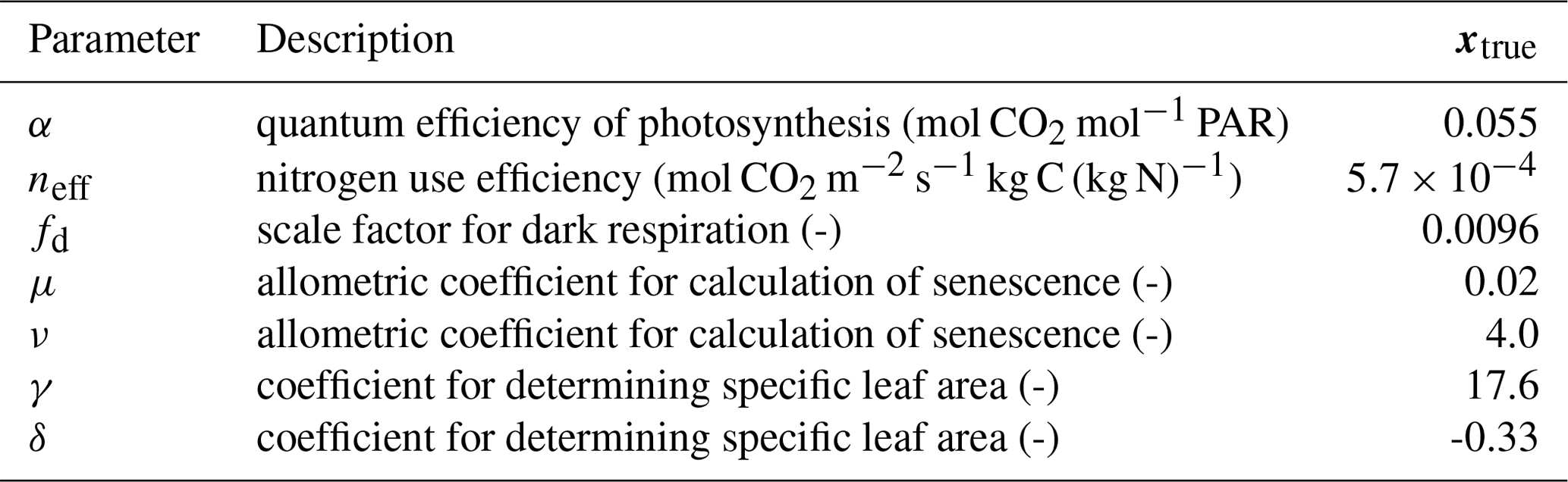
Table 1Description of parameters optimized in experiments and model truth value. PAR represents photosynthetically active radiation.
To use another model in this framework, new wrappers would have to be written to mimic the functionality of jules.py and run_jules.py and allow for multiple model runs to be conducted while varying parameters. The module run_experiment.py would need to be updated to account for these new wrappers and functions to extract the observations for assimilation included in experiment_setup.py. Although we have used Python here to implement a stand-alone setup of LAVENDAR, we envisage that the technique could be added to existing workflow systems such as Cylc (Oliver et al., 2019) or the Predictive Ecosystem Analyzer (PEcAn) (LeBauer et al., 2013).
2.3.4 Tests of the four-dimensional ensemble variational data assimilation system
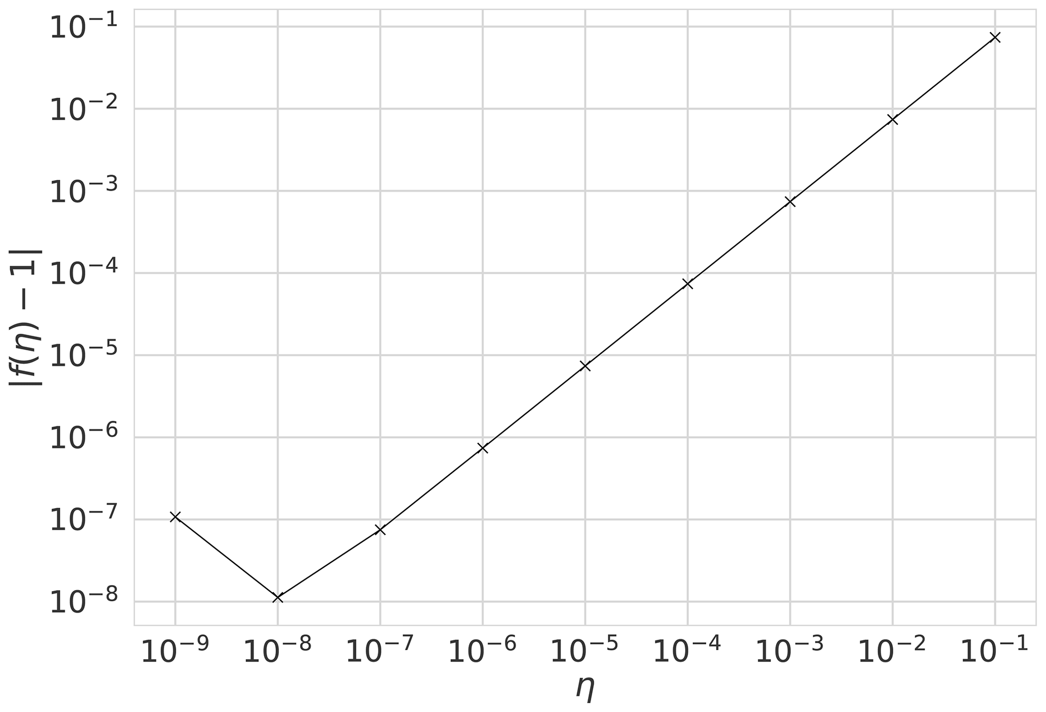
It is important to ensure correctness of the 4D-En-Var system. We show that our system is correct and passes tests for the gradient of the cost function (Li et al., 1994; Navon et al., 1992). For the cost function J and its gradient ∇J, we show that our implementation of ∇J is correct using the identity,
where b is a vector of unit length and η is a parameter controlling the size of b. For small values of η we should find f(η) close to 1. Figure 1 shows for a year's assimilation window with where w is calculated from the prior parameter values (see Table 3) perturbed by 30 %. We can see that as η→0 as expected, until f(η) gets too close to machine precision at . This was also tested with different choices of b finding similar results.
2.4 Experiments
2.4.1 Twin experiments
A so-called “twin” experiment in data assimilation is one where a model is used to generate synthetic observations to be assimilated. This is a commonly used approach to test whether particular combinations of observations can, in principle, be used to retrieve desired target variables using some DA method. In effect the model that the observations are being assimilated into is “perfect” because it represents the underlying physics that gave rise to them in the first place. We conducted a parameter estimation twin experiment with the aim to recover values for key JULES-crop parameters: the quantum efficiency of photosynthesis, nitrogen use efficiency (scale factor relating Vcmax with leaf nitrogen concentration), scale factor for dark respiration, two allometric coefficients for calculation of senescence and two coefficients for determining specific leaf area (see Table 1). These seven parameters have an effect on the crop's seasonal growth cycle and its photosynthetic response to meteorological forcing data. The choice of parameters was motivated by the analysis of Williams et al. (2017), who found that they were least able to constrain these parameters with the available data. We assimilated synthetic observations of gross primary productivity (GPP), leaf area index (LAI) and canopy height, all generated by JULES, over a year-long assimilation window.
The model truth was taken from the values given in Williams et al. (2017) and perturbed using a normal distribution with a 10 % standard deviation to find a prior parameter vector, xb. We then generated an ensemble by drawing 50 parameter vectors from the normal distribution with mean xb and variance (0.15×xb)2. Synthetic observations were sampled from the model truth with the same frequency as the real observations available from Mead and perturbed using Gaussian noise with a standard deviation of 2 % of the synthetic truth value. This provided an idealized test case where we have high confidence in the assimilated observations to ensure our system is working and can recover a set of known parameters, given known prior and observation error statistics. We also include a twin experiment using the same error statistics as those used for the real data experiments at the Mead site (outlined in Sect. 2.4.2) in Supplement Sect. S1.1.
2.4.2 Mead experiments
For the experiments using real data from the Mead US-Ne1 FLUXNET site, the same seven parameters were optimized (shown in Table 1) by assimilating observations over a year-long assimilation window in 2008. The prior parameter vector, xb, is taken from the values given in Williams et al. (2017). We then generated an ensemble of 50 parameter vectors by sampling from the normal distribution with mean xb and variance (0.25×xb)2. We apply the same variance to all parameters here as the analysis of Williams et al. (2017) showed these parameters to all be poorly constrained with the available data in a more traditional model calibration study. In reality it is unlikely that all parameters will have the same variance but in the absence of additional information and for the purposes of this demonstration we used (0.25×xb)2. Observations for the site are described in Sect. 2.2. We prescribe a 5 % standard deviation for canopy height and leaf area index errors and a 10 % standard deviation for errors in GPP. These uncertainties are rough estimates that we considered adequate for demonstrating our system, but for any specific application the errors estimates should be determined more carefully. However, our uncertainties are consistent with Schaefer et al. (2012), who found an uncertainty of 1.04 to 4.15 g C m−2 d−1 (scaling with flux magnitude) for estimates of GPP; Raj et al. (2016), who found an uncertainty of the order of 10 % for daily estimates of GPP; and Guindin-Garcia et al. (2012), who found a standard error of 0.15 m2 m−2 for destructively sampled green LAI at the Mead flux site. The error statistics used within the data assimilation experiments could be investigated more thoroughly but are appropriate for demonstrating the validity of the technique and providing an optimal weighting between prior and observation estimates.
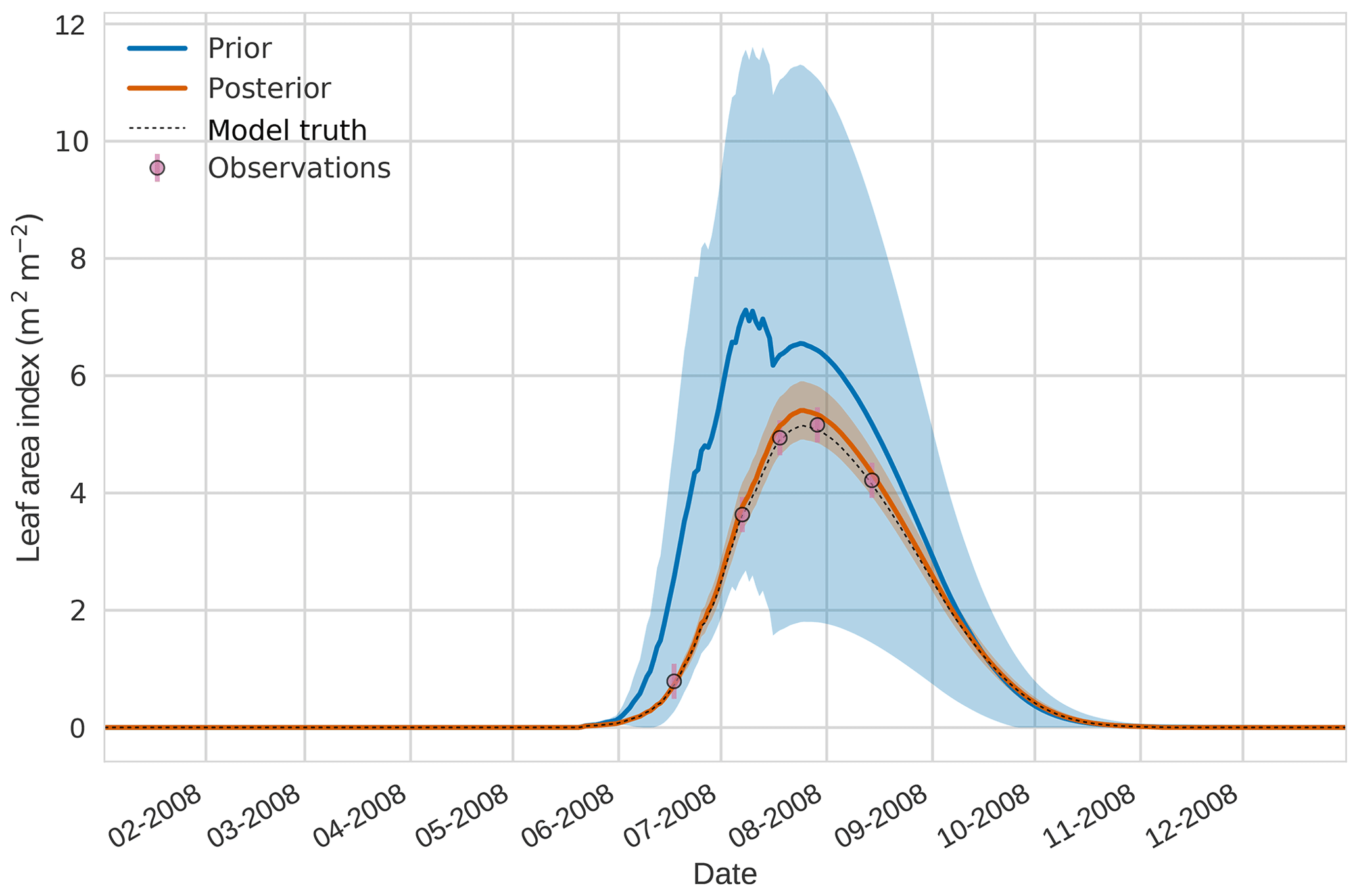
Figure 2 4D-En-Var twin results for leaf area index using 50 ensemble members. Blue shading: prior ensemble spread (), orange shading: posterior ensemble spread (±1σ), pink dots: observations with error bars, dashed black line: model truth.
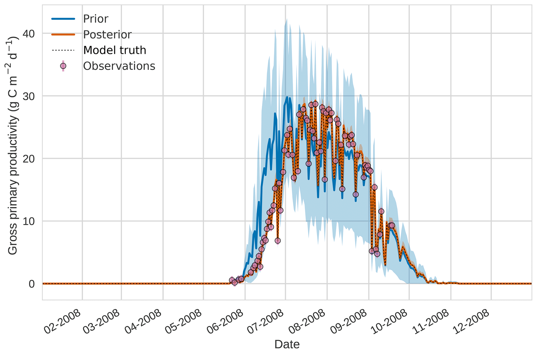
Figure 3 4D-En-Var twin results for gross primary productivity using 50 ensemble members. Blue shading: prior ensemble spread (±1σ), orange shading: posterior ensemble spread (±1σ), pink dots: observations with error bars, dashed black line: model truth.
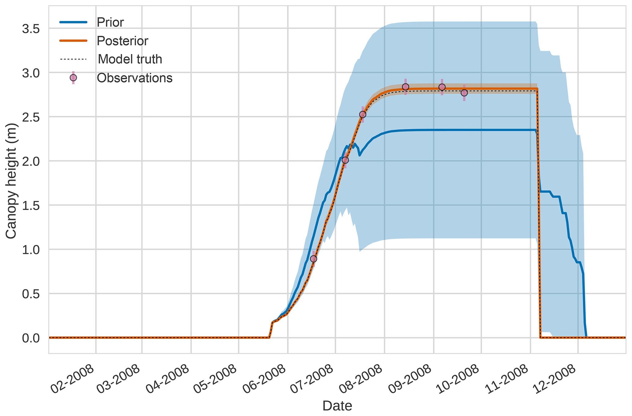
Figure 4 4D-En-Var twin results for canopy height using 50 ensemble members. Blue shading: prior ensemble spread (±1σ), orange shading: posterior ensemble spread (±1σ), pink dots: observations with error bars, dash black line: model truth.
3.1 Twin experiments
Figures 2 to 4 show plots of the three target variables over the year-long assimilation window. For these figures the blue line and shading represent the 50 member prior ensemble mean and spread (±1 standard deviation), the orange line and corresponding shading represent the same but for the 50 member posterior ensemble of JULES model runs, pink dots with vertical lines are the synthetic observations with error bars (±1 standard deviation) and the dashed black line is the trajectory of the JULES model using the “true” parameter values. Figure 2 shows that after data assimilation the posterior model estimate tracks the model truth trajectory closely with the LAI model truth always being captured by the posterior ensemble spread. For GPP, Fig. 3 shows a very similar result as for LAI with the posterior estimate fully capturing the model truth. Figure 4 illustrates the effect the large spread of the prior ensemble has on harvest dates towards the end of the season, with the ensemble spread increasing markedly as different ensemble members are harvested on different days. The spread for the posterior estimate of canopy height reduces considerably and tracks the model truth well. Figure 5 shows prior, posterior and true trajectories for harvestable material. We have not assimilated any observations of this quantity but this figure shows we improve predictions of harvestable material after assimilation of the three previously discussed target variables. In Table 2 we show root-mean-square error (RMSE) for the three target variables before and after assimilation. We find an average 93.67 % reduction in RMSE for the three target variables.
Table 24D-En-Var twin assimilated observation RMSE for the four target variables when an ensemble of size 50 is used in experiments.
Prior and posterior distributions for the seven parameters are shown in Fig. 6 (light grey and dark grey, respectively) with the true model parameter values shown as dashed black vertical lines. For all seven parameters, the posterior distribution moves toward the model truth and in most cases the posterior distribution mean appears very close to the model truth. The posterior distributions also narrow significantly in comparison to the prior distributions with the exception of fd. Table 3 shows the mean prior and posterior parameter vectors and percentage error values between prior parameter estimates and the model truth and posterior parameter estimates and the model truth. The percentage error in the posterior estimate is reduced for all parameters, again with the exception of fd. The inability of the technique to recover fd is discussed further in Sect. 4.1. There is an average error of 10.32 % in the prior parameter estimates and this is reduced to 2.93 % for the posterior estimates.
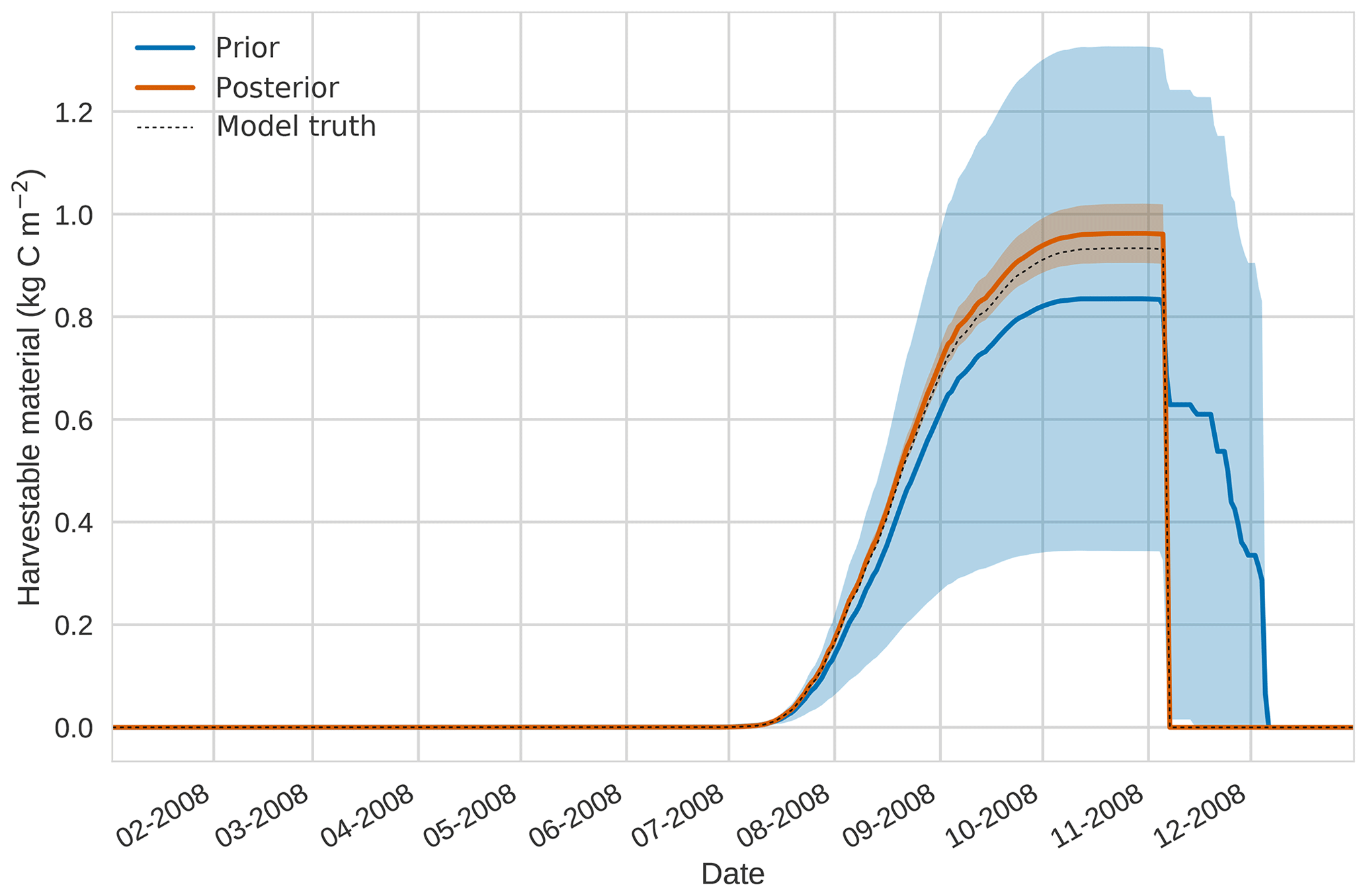
Figure 5 4D-En-Var twin results for harvestable material using 50 ensemble members. Blue shading: prior ensemble spread (±1σ), orange shading: posterior ensemble spread (±1σ), pink dots: observations with error bars, dashed black line: model truth.

Figure 6 4D-En-Var twin distributions for the seven optimized parameters for both the prior ensemble (light grey) and posterior ensemble (dark grey). The value of the model truth is shown as a dashed vertical black line.
Table 34D-En-Var twin results and percentage error for each of the seven optimized parameters when an ensemble of size 50 is used in experiments.
3.2 Mead field observations
Figures 7 to 9 show assimilation results for the three target variables over the year-long window for the Mead field site. For these figures, the blue line and shading represent the 50 member prior ensemble mean (taken from Williams et al., 2017) and spread (±1 standard deviation), the orange line and shading represent the same but for the 50-member posterior ensemble of JULES model runs after data assimilation and the pink dots with vertical lines are the field observations from Mead site US-Ne1 with error bars (±1 standard deviation). From Fig. 7 we can see that the prior mean underestimates LAI, reaching a much lower peak than observations; despite this, the technique finds a posterior mean estimate that agrees well with all but two LAI observations (in September and October). We find similar results for GPP in Fig. 8, with the posterior capturing the majority of observations but missing some of the highest values. For canopy height in Fig. 9, the effect of the spread in ensemble harvest dates for the prior is again obvious (also seen in the twin experiments, Fig. 4); this spread is reduced for the posterior estimate and all observations are captured by the posterior ensemble spread.
Prior and posterior estimates for unassimilated independent observations are shown in Figs. 10 to 12. From Fig. 10 we can see the prior estimate is underestimating the amount of harvestable material for the maize crop. After assimilation the posterior estimate predicts the amount of harvestable material well and with increased confidence. Figure 11 shows that our posterior estimate of leaf carbon content improves after assimilation but is still too low; this is the same for stem carbon content in Fig. 12. The fact that we can find good agreement for LAI with a poorer fit to leaf carbon content is likely due to the optimized parameters controlling specific leaf area compensating for errors in model parameters controlling the partitioning of net primary productivity into the leaf carbon pool. This allows us to achieve the correct leaf area with the incorrect leaf carbon content.
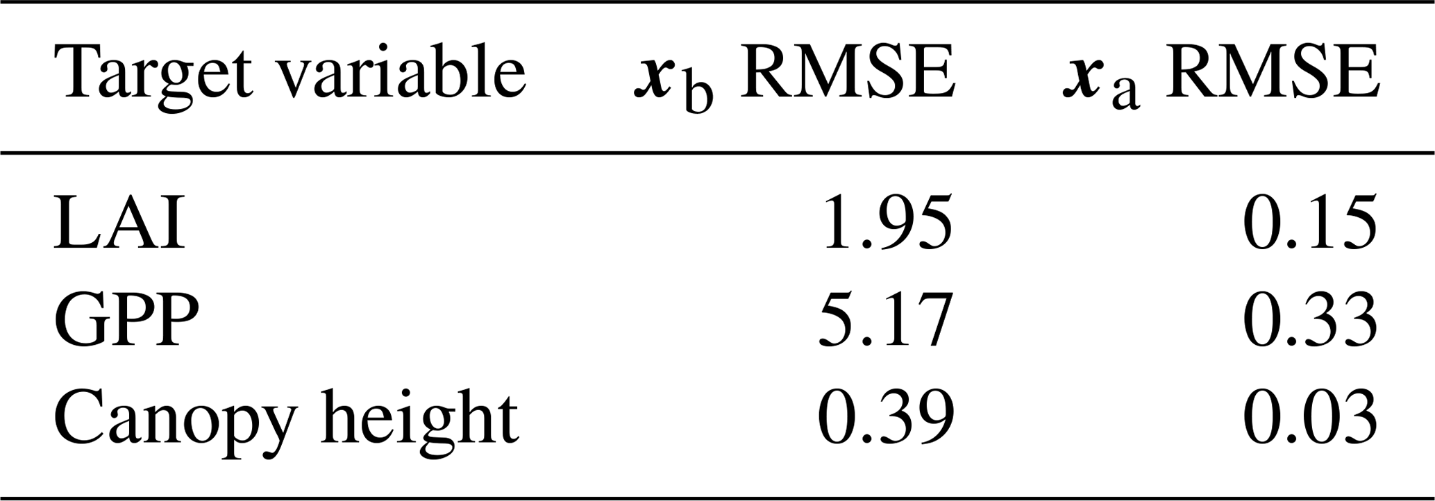
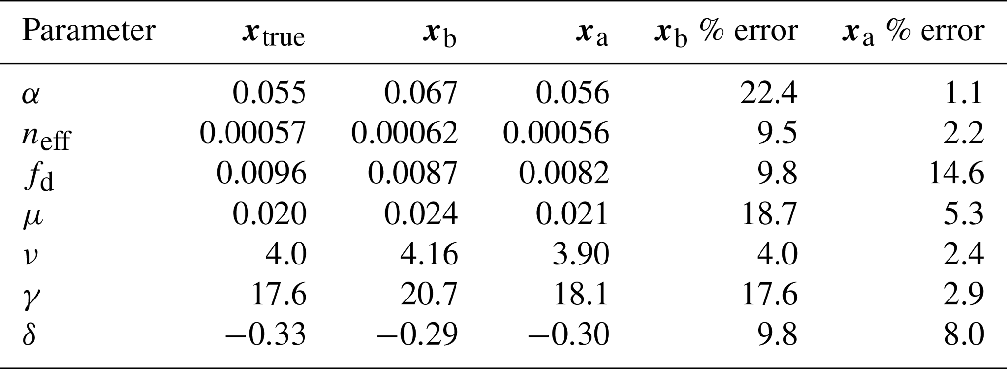
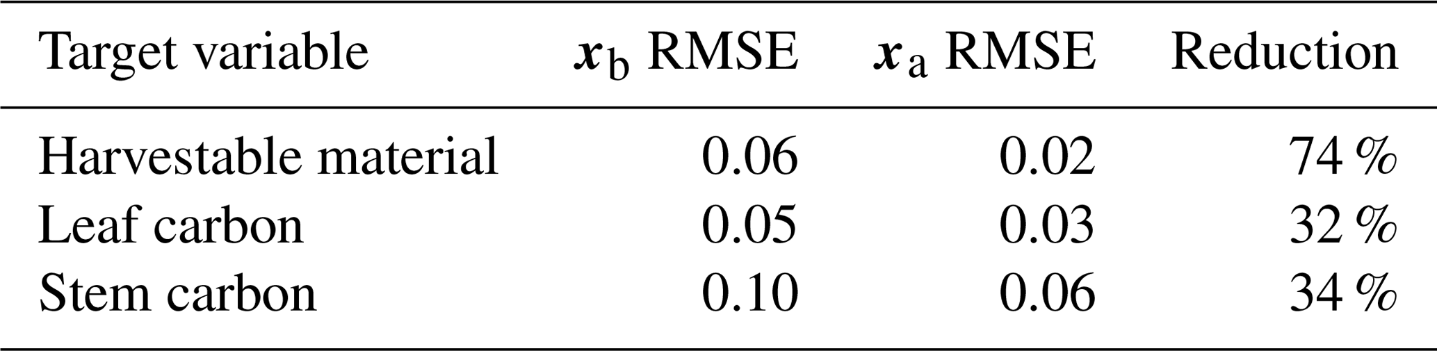
Prior and posterior ensemble parameter distributions are shown in Fig. 13. After assimilation the distributions have shifted and narrowed for all parameters, except fd, with α being the most extreme example of this. The effect these updated parameter distributions have on the model prediction of the three target variables in Table 4 is clear. We find the largest reduction in RMSE for canopy height (73 %) with the smallest reduction in RMSE for GPP (44 %); overall, we found an average 59 % reduction in RMSE for the three target variables. From Table 5 we can see the updated parameters have also reduced the model prediction RMSE in independent unassimilated observations. The largest reduction is in the prediction of harvestable material (74 %); overall, we have found an average 47 % reduction in RMSE for the three independent observation types.
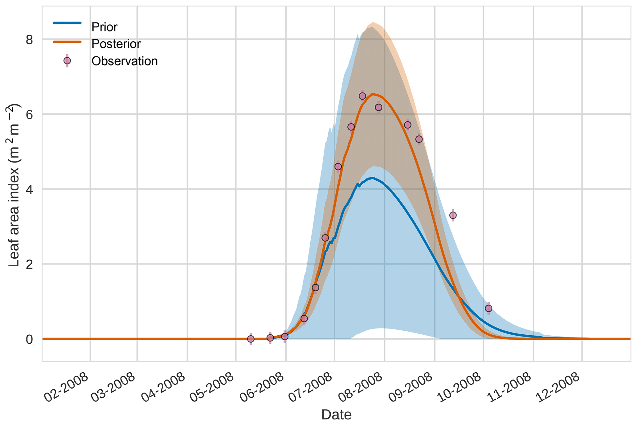
Figure 74D-En-Var results for leaf area index using 50 ensemble members. Blue shading: prior ensemble spread (±1σ), orange shading: posterior ensemble spread (±1σ), pink dots: observations with error bars.
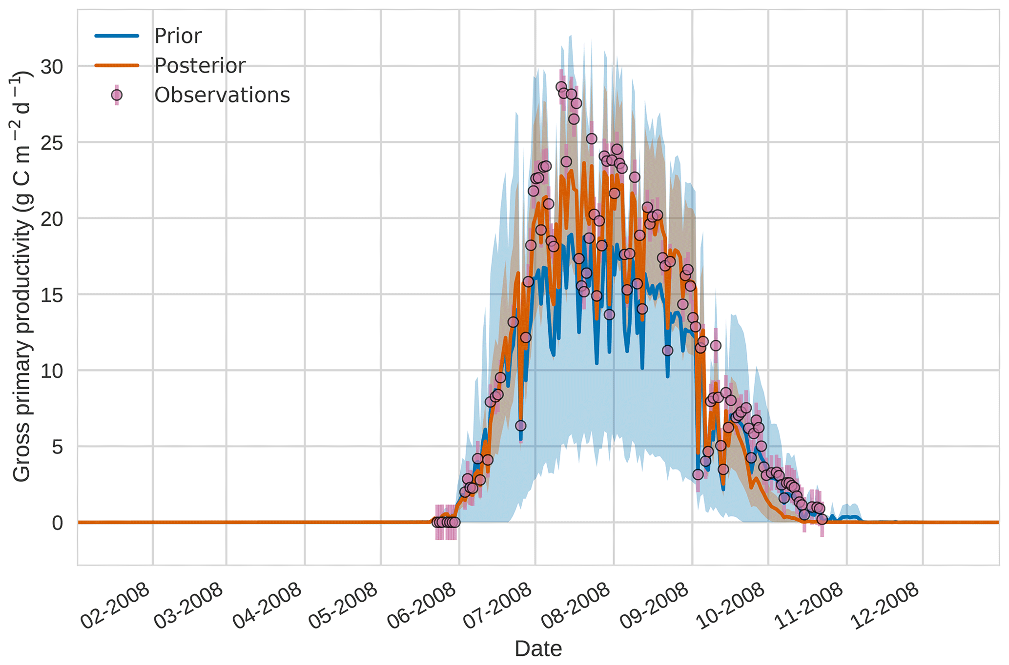
Figure 84D-En-Var results for gross primary productivity using 50 ensemble members. Blue shading: prior ensemble spread (±1σ), orange shading: posterior ensemble spread (±1σ), pink dots: observations with error bars.
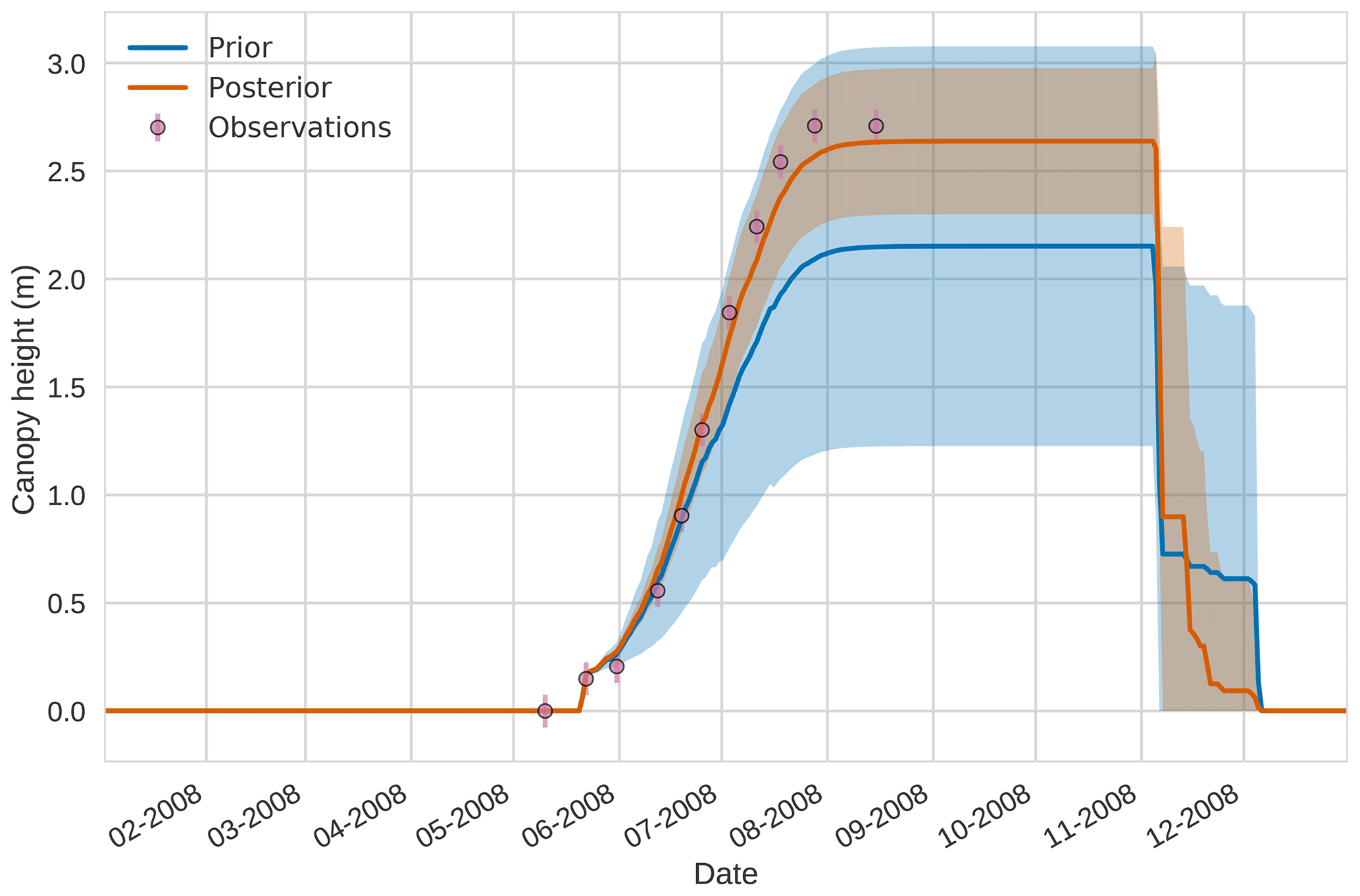
Figure 94D-En-Var results for canopy height using 50 ensemble members. Blue shading: prior ensemble spread (±1σ), orange shading: posterior ensemble spread (±1σ), pink dots: observations with error bars.

Figure 104D-En-Var results for harvestable material using 50 ensemble members. Blue shading: prior ensemble spread (±1σ), orange shading: posterior ensemble spread (±1σ), pink dots: observations.
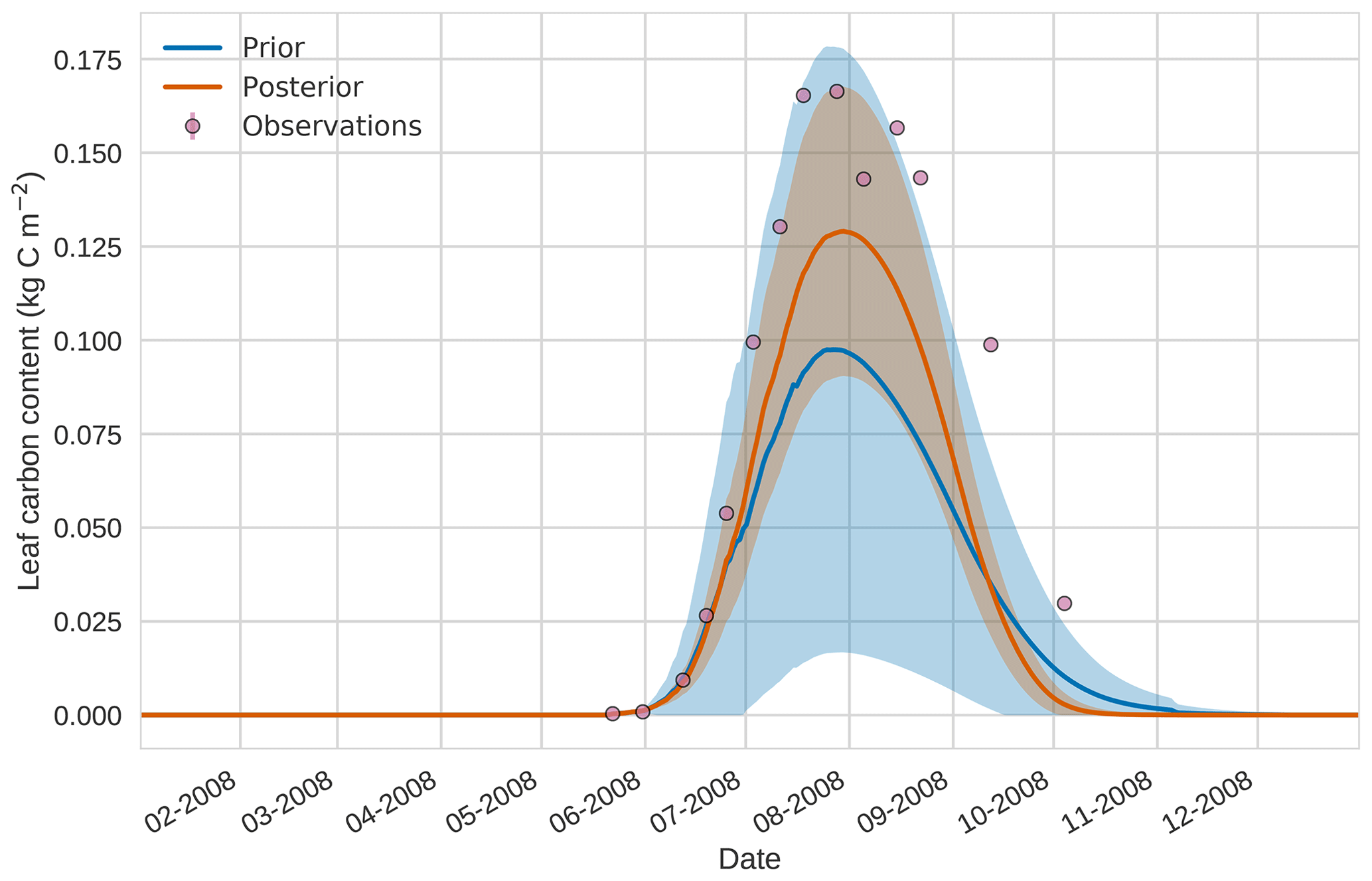
Figure 114D-En-Var results for leaf carbon using 50 ensemble members. Blue shading: prior ensemble spread (±1σ), orange shading: posterior ensemble spread (±1σ), pink dots: observations.
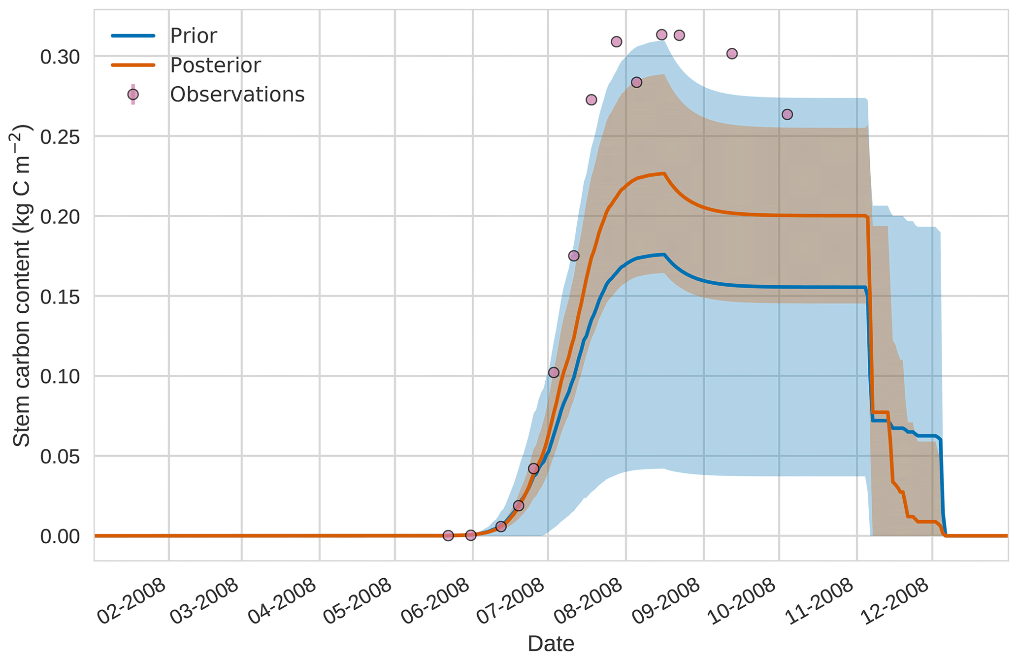
Figure 124D-En-Var results for stem carbon using 50 ensemble members. Blue shading: prior ensemble spread (±1σ), orange shading: posterior ensemble spread (±1σ), pink dots: observations.
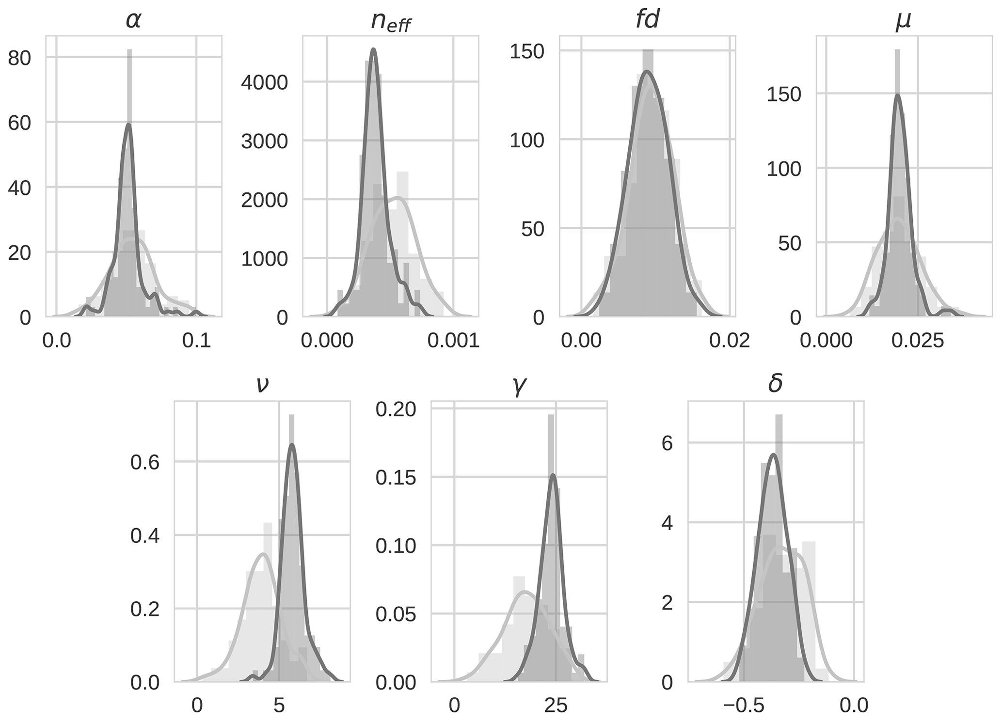
Figure 134D-En-Var distributions for the seven optimized parameters for both the prior ensemble (light grey) and posterior ensemble (dark grey).
Table 44D-En-Var Mead assimilated observation RMSE for the three target variables when an ensemble of size 50 is used in experiments.
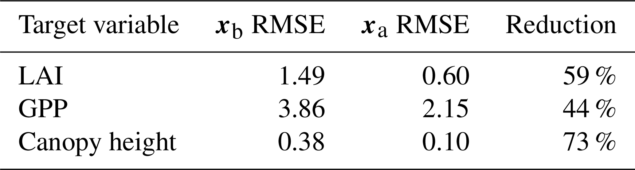
Table 54D-En-Var Mead unassimilated observation RMSE when an ensemble of size 50 is used in experiments.
4.1 Twin experiments
In Sect. 3.1 we have demonstrated that the 4D-En-Var technique is able to retrieve a synthetic truth given known prior and observation error statistics. There is good agreement between the mean posterior trajectory and model truth for the three target variables (see Figs. 2, 3 and 4). We also retrieve accurate predictions of independent unobserved quantities such as harvestable material (see Fig. 5). The mean posterior parameter vector after assimilation is very close to the model truth as shown in Table 3 and Fig. 13 with the exception of the scale factor for dark respiration fd. Our inability to recover this parameter is likely due to the fact that the assimilated daily averaged observations are not greatly impacted by changes in dark respiration. Assimilating total aboveground carbon could improve the estimation of fd by giving us a proxy to the net primary productivity of the crop and with the concurrent assimilation of GPP a better constraint on respiration. Alternatively, including correlations in the prior error covariance matrix would provide information to update fd even when the assimilated observations are not impacted by changes in this parameter. It has been shown that suitable correlations can be diagnosed by sampling from a set of predetermined ecological dynamical constraints and taking the covariance of an ensemble run forward over a set time window (Pinnington et al., 2016).
In the results for all predicted variables we find that the posterior ensemble converges around the model truth. This can also be seen for the parameters in Fig. 6, where the posterior ensemble spread of the parameter α is particularly narrow. This could lead to problems when using our posterior estimate as the prior for a new assimilation cycle. It is also possible that equifinality could become an issue when attempting to optimize a larger number of parameters. From Table 3 we can see this issue for the two parameters controlling photosynthetic response with the posterior slightly over-predicting α and under-predicting neff, as different combinations of these parameters can produce the same trajectory for the observed target variables. The effect of equifinality can be seen more clearly for the posterior ensemble correlation matrix included in Fig. S7 in the Supplement. It is also clear that selection of the prior ensemble is important to the success of the technique. From Figs. 4 and 5 it can be seen that the prior ensemble is poor, suggesting that it could be better conditioned to deal with the discontinuity of the harvest date. It may be the case that for more complex problems an iterative step in the assimilation would be needed to address this (Bocquet, 2015) or ensemble localization in time. In this study we have only considered the uncertainty in the parameters and initial conditions and not the uncertainty in forcing data, random effects (parameter variability) or uncertainty in the process model (Dietze, 2017). The inclusion of these additional sources of error would avoid the ensemble converging too tightly around any given value. In order to include uncertainty in the forcing data, it would be necessary to run each ensemble member with a different realization of the driving meteorology. Process error could be included in Eq. (5) resulting in a new term in the 4D-En-Var cost function in Eq. (24), containing a model error covariance matrix; it has also been shown that these different types of uncertainty could be built into the observation error covariance matrix R (Howes et al., 2017). If estimates to these sources of error are not available, the use of methods such as ensemble inflation (Anderson and Anderson, 1999), a set of techniques where the ensemble spread is artificially inflated, will help alleviate problems of ensemble convergence.
4.2 Mead field observations
We have demonstrated the ability of the technique to improve JULES model predictions using real data in Sect. 3.2. Posterior estimates improve the fit to observations with the posterior ensemble spread capturing the majority of assimilated observations (see Figs. 7, 8 and 9). We reduce the RMSE in the mean model prediction by an average of 59 % for the three target variables. As independent validation that we are improving the skill of the JULES model, we also improve the fit to three unassimilated observation types (see Figs. 10, 11 and 12) with an average reduction in RMSE of 47 %. We find the largest reduction in RMSE for the independent observations for harvestable material (74 % reduction), which is an important variable closely linked to crop yield. The improvement in skill for the unassimilated observations gives us confidence that the technique has updated the model parameters in a physically realistic way and that we have not over-fitted the assimilated data. By conducting a hindcast for 2009 (shown in the Supplement Fig. S6 and Table S2), we also find the retrieved posterior ensemble improves the fit to the unassimilated observations in the subsequent year, with an average reduction in RMSE of 54 % when compared with the prior estimate.
The experiments with Mead field observations do not show the same level of reduction in ensemble spread as in the twin experiments (see Fig. 13) due to the specified prior and observation errors being much larger. However, the posterior distribution for some parameters is still quite narrow. We again find very little update for fd as in the twin experiments, suggesting that the assimilated observations (at their current temporal resolution) are not sensitive to changes in this parameter. In our experiments we have held back observations of harvestable material, leaf carbon and stem carbon to use as independent validation of the technique. However, these observations could have been included in the assimilation to better constrain the current parameters or consider a larger parameter set.
4.3 Challenges and opportunities
Avoiding the computation of an adjoint makes the technique of 4D-En-Var much easier to implement and also agnostic about the land surface model used. By maintaining a variational approach and optimizing parameters over a time window against all available observations, we also avoid retrieving non-physical time-varying parameters associated with more common sequential ensemble methods. However, as with other ensemble techniques, results are dependent on having a well conditioned prior ensemble. Methods of ensemble localization (Hamill et al., 2001), where distant correlations or ensemble members are down-weighted or removed, could be used to improve prior estimates. In this instance we would need to consider localization in time (Bocquet, 2015). In order to extend this framework to model runs over a spatial grid we will need a method to sample prior parameter distributions regionally or globally, it would then be possible to conduct parameter estimation experiments over a region, either on a point-by-point basis or for the whole area at once. Considering a large area would increase the parameter space and require more ensemble members. Localization in space could help to reduce the parameter space and thus allow for use of a smaller ensemble. The ensemble aspect of the technique also allows us to retrieve posterior distributions of parameters, whereas in pure variational methods we would only find a posterior mean. However, this also presents a possible issue of posterior ensemble convergence around certain parameters. Including additional sources of error within the assimilation system (driving data error, parameter variability, process error) or using methods such as inflation (Anderson and Anderson, 1999) will help to avoid this and ensure our posterior estimates maintain enough spread to be used as a prior estimate in new assimilation cycles. While posterior parameter estimates could be used in future studies with their associated uncertainties, we envisage that cycling of the assimilation system will be more appropriate for state estimation (after initial parameter estimation) where the system could be cycled on a timescale suitable for the required state variable and data availability.
In 4D-En-Var we approximate the tangent linear model using an ensemble perturbation matrix. Without the explicit knowledge of the tangent linear and adjoint models 4D-En-Var could be less able to deal with non-linearities in the process model in cases where the ensemble is small or ill-conditioned. For the examples presented in this paper 4D-En-Var deals well with the non-linearity of the JULES land surface model. However, it is possible that for high dimensional spaces, a technique of stochastic ensemble iteration (Bocquet and Sakov, 2013) will need to be implemented to cope with increased non-linearity at the cost of multiple model runs within the minimization routine. The framework proposed in this paper allows for the implementation of such a technique fairly easily.
In this paper we have focused on using LAVENDAR for parameter estimation. However, the technique we present can just as easily be used to adjust the model state at the start of an assimilation window in much the same way as is done in weather forecasting (Liu et al., 2008). In this case it is likely that a shorter assimilation window would be required. The posterior ensemble is then used to provide the initial conditions for the next assimilation window. This would require additional modules to be written within LAVENDAR, which would handle the starting and stopping of the process model. It would also require that the implemented model was able to dump the full existing model state and then be restarted with an updated version of this state (as is possible with JULES). In this iterative framework accounting for model error would also become more important.
A particularly appealing aspect of LAVENDAR as presented in this paper is that there is no interaction between the DA technique and the model itself – once the initial ensemble is generated it is not necessary to run the model again to perform any aspect of the DA. Because the main computational overhead is running the model, this makes the DA analysis extremely efficient. This is quite unlike related techniques such as 4D-Var and provides some unique opportunities. For example, it lends itself to efficient implementation of Observing System Simulation Experiments (OSSEs). OSSEs are used to examine the impact of different observation networks and sampling strategies on specific model data assimilation problems by repeating twin experiments with different sets of synthetic observations used to mimic different instruments and/or sampling regimes. In LAVENDAR the synthetic observations for a large number of different scenarios can all be generated with the initial ensemble and hence facilitate a large number of OSSE experiments without any further model runs.
Variational DA with land surface models holds a lot of potential, especially for parameter estimation, but as land surface models become more complex and subject to more frequent version releases the calculation and maintenance of a model adjoint will become increasingly expensive. One way to avoid the computation of a model adjoint is to move to ensemble data assimilation methods. In this paper we have documented LAVENDAR for the implementation of 4D-En-Var data assimilation with land surface models. We have shown the application of LAVENDAR to the JULES land surface model, but as it requires no modification to the model itself it can easily be applied to any land surface model. Using LAVENDAR with JULES we retrieved a set of true model parameters given known prior and observation error statistics in a set of twin experiments and improved model predictions of real-world observations from the Mead continuous maize US-Ne1 FLUXNET site. The use of 4D-En-Var with land models holds a great deal of potential for both parameter and state estimation. The additional computational overhead compared to 4D-Var is an appealing compromise given the simplicity and generality of its implementation.
The code and documentation used for the experiments in this paper are available from https://github.com/pyearthsci/lavendar (last access: 20 February 2019) (Pinnington, 2019). Data for the Mead site US-Ne1 are available from http://fluxnet.fluxdata.org/ (last access: 6 January 2020; Fluxdata, 2017).
EP, TQ and KW designed the experiments. AL provided advice on the data assimilation technique and tests. EP developed the data assimilation code and performed the simulations. TA and DS provided observations from the Mead US-Ne1 site. EP prepared the article with contributions from all co-authors.
The authors declare that they have no conflict of interest.
This work was funded by the UK Natural Environment Research Council's National Centre for Earth Observation ODA programme (NE/R000115/1). The US-Ne1, US-Ne2 and US-Ne3 AmeriFlux sites are supported by the Lawrence Berkeley National Lab AmeriFlux Data Management Program and by the Carbon Sequestration Program, University of Nebraska-Lincoln Agricultural Research Division. Funding for AmeriFlux core site data was provided by the U.S. Department of Energy’s Office of Science. Partial support from the Nebraska Agricultural Experiment Station with funding from the Hatch Act (accession number 1002649) through the USDA National Institute of Food and Agriculture is also acknowledged.
This research has been supported by the Natural Environment Research Council (grant no. NE/R000115/1).
This paper was edited by Adrian Sandu and reviewed by two anonymous referees.
Anderson, J. L. and Anderson, S. L.: A Monte Carlo Implementation of the Nonlinear Filtering Problem to Produce Ensemble Assimilations and Forecasts, Mon. Weather Rev., 127, 2741–2758, https://doi.org/10.1175/1520-0493(1999)127<2741:AMCIOT>2.0.CO;2, 1999. a, b
Bacour, C., Peylin, P., MacBean, N., Rayner, P. J., Delage, F., Chevallier, F., Weiss, M., Demarty, J., Santaren, D., Baret, F., Berveiller, D., Dufrêne, E., and Prunet, P.: Joint assimilation of eddy-covariance flux measurements and FAPAR products over temperate forests within a process-oriented biosphere model, J. Geophys. Res.-Biogeosci., 120, 1839–1857, https://doi.org/10.1002/2015JG002966, 2015. a
Bannister, R. N.: A review of operational methods of variational and ensemble-variational data assimilation, Q. J. Roy. Meteorol. Soc., 143, 607–633, https://doi.org/10.1002/qj.2982, 2016. a, b
Best, M. J., Pryor, M., Clark, D. B., Rooney, G. G., Essery, R. L. H., Ménard, C. B., Edwards, J. M., Hendry, M. A., Porson, A., Gedney, N., Mercado, L. M., Sitch, S., Blyth, E., Boucher, O., Cox, P. M., Grimmond, C. S. B., and Harding, R. J.: The Joint UK Land Environment Simulator (JULES), model description – Part 1: Energy and water fluxes, Geosci. Model Dev., 4, 677–699, https://doi.org/10.5194/gmd-4-677-2011, 2011. a, b
Bloom, A. A. and Williams, M.: Constraining ecosystem carbon dynamics in a data-limited world: integrating ecological “common sense” in a model-data fusion framework, Biogeosciences, 12, 1299–1315, https://doi.org/10.5194/bg-12-1299-2015, 2015. a
Bloom, A. A., Exbrayat, J.-F., van der Velde, I. R., Feng, L., and Williams, M.: The decadal state of the terrestrial carbon cycle: Global retrievals of terrestrial carbon allocation, pools, and residence times, P. Natl. Acad. Sci., 113, 1285–1290, 2016. a
Bocquet, M.: Localization and the iterative ensemble Kalman smoother, Q. J. Roy. Meteorol. Soc., 142, 1075–1089, https://doi.org/10.1002/qj.2711, 2015. a, b
Bocquet, M. and Sakov, P.: Joint state and parameter estimation with an iterative ensemble Kalman smoother, Nonlin. Processes Geophys., 20, 803–818, https://doi.org/10.5194/npg-20-803-2013, 2013. a
Bocquet, M. and Sakov, P.: An iterative ensemble Kalman smoother, Q. J. Roy. Meteorol. Soc., 140, 1521–1535, https://doi.org/10.1002/qj.2236, 2014. a
Braswell, B. H., Sacks, W. J., Linder, E., and Schimel, D. S.: Estimating diurnal to annual ecosystem parameters by synthesis of a carbon flux model with eddy covariance net ecosystem exchange observations, Global Change Biol., 11, 335–355, 2005. a
Clark, D. B., Mercado, L. M., Sitch, S., Jones, C. D., Gedney, N., Best, M. J., Pryor, M., Rooney, G. G., Essery, R. L. H., Blyth, E., Boucher, O., Harding, R. J., Huntingford, C., and Cox, P. M.: The Joint UK Land Environment Simulator (JULES), model description – Part 2: Carbon fluxes and vegetation dynamics, Geosci. Model Dev., 4, 701–722, https://doi.org/10.5194/gmd-4-701-2011, 2011. a, b
De Lannoy, G. J. M. and Reichle, R. H.: Assimilation of SMOS brightness temperatures or soil moisture retrievals into a land surface model, Hydrol. Earth Syst. Sci., 20, 4895–4911, https://doi.org/10.5194/hess-20-4895-2016, 2016. a
Desroziers, G., Camino, J.-T., and Berre, L.: 4DEnVar: link with 4D state formulation of variational assimilation and different possible implementations, Q. J. Roy. Meteorol. Soc., 140, 2097–2110, https://doi.org/10.1002/qj.2325, 2014. a
Dietze, M. C.: Prediction in ecology: a first-principles framework, Ecol. Appl., 27, 2048–2060, https://doi.org/10.1002/eap.1589, 2017. a
Evensen, G.: The Ensemble Kalman Filter: theoretical formulation and practical implementation, Ocean Dynam., 53, 343–367, https://doi.org/10.1007/s10236-003-0036-9, 2003. a
Fer, I., Kelly, R., Moorcroft, P. R., Richardson, A. D., Cowdery, E. M., and Dietze, M. C.: Linking big models to big data: efficient ecosystem model calibration through Bayesian model emulation, Biogeosciences, 15, 5801–5830, https://doi.org/10.5194/bg-15-5801-2018, 2018. a
Fluxdata: The Data Portal serving the FLUXNET community, Lawrence Berkeley National Laboratory, available at: http://fluxnet.fluxdata.org/ (last access: 6 January 2020), 2017. a
Ghent, D., Kaduk, J., Remedios, J., Ardö, J., and Balzter, H.: Assimilation of land surface temperature into the land surface model JULES with an ensemble Kalman filter, J. Geophys. Res.-Atmos., 115, D19112, https://doi.org/10.1029/2010JD014392, 2010. a
Gómez-Dans, J. L., Lewis, P. E., and Disney, M.: Efficient Emulation of Radiative Transfer Codes Using Gaussian Processes and Application to Land Surface Parameter Inferences, Remote Sens., 8, https://doi.org/10.3390/rs8020119, 2016. a
Guindin-Garcia, N., Gitelson, A. A., Arkebauer, T. J., Shanahan, J., and Weiss, A.: An evaluation of MODIS 8- and 16-day composite products for monitoring maize green leaf area index, Agr. Forest Meteorol., 161, 15–25, https://doi.org/10.1016/j.agrformet.2012.03.012, 2012. a, b
Hamill, T. M., Whitaker, J. S., and Snyder, C.: Distance-Dependent Filtering of Background Error Covariance Estimates in an Ensemble Kalman Filter, Mon. Weather Rev., 129, 2776–2790, https://doi.org/10.1175/1520-0493(2001)129<2776:DDFOBE>2.0.CO;2, 2001. a
Howes, K. E., Fowler, A. M., and Lawless, A. S.: Accounting for model error in strong-constraint 4D-Var data assimilation, Q. J. Roy. Meteorol. Soc., 143, 1227–1240, https://doi.org/10.1002/qj.2996, 2017. a
Keenan, T. F., Davidson, E., Moffat, A. M., Munger, W., and Richardson, A. D.: Using model-data fusion to interpret past trends, and quantify uncertainties in future projections, of terrestrial ecosystem carbon cycling, Global Change Biol., 18, 2555–2569, https://doi.org/10.1111/j.1365-2486.2012.02684.x, 2012. a
Kolassa, J., Reichle, R., and Draper, C.: Merging active and passive microwave observations in soil moisture data assimilation, Remote Sens. Environ., 191, 117–130, 2017. a
LeBauer, D., Wang, D., Richter, K., Davidson, C., and Dietze, M.: Facilitating feedbacks between field measurements and ecosystem models, Ecol. Mono., 83, 133–154, https://doi.org/10.1890/12-0137.1, 2013. a
Li, Y., Navon, I. M., Yang, W., Zou, X., Bates, J. R., Moorthi, S., and Higgins, R. W.: Four-Dimensional Variational Data Assimilation Experiments with a Multilevel Semi-Lagrangian Semi-Implicit General Circulation Model, Mon. Weather Rev., 122, 966–983, https://doi.org/10.1175/1520-0493(1994)122<0966:FDVDAE>2.0.CO;2, 1994. a
Liu, C., Xiao, Q., and Wang, B.: An Ensemble-Based Four-Dimensional Variational Data Assimilation Scheme. Part I: Technical Formulation and Preliminary Test, Mon. Weather Rev., 136, 3363–3373, https://doi.org/10.1175/2008MWR2312.1, 2008. a, b, c
Luo, Y., Keenan, T. F., and Smith, M.: Predictability of the terrestrial carbon cycle, Global Change Biol., 21, 1737–1751, https://doi.org/10.1111/gcb.12766, 2015. a
Metropolis, N., Rosenbluth, A. W., Rosenbluth, M. N., Teller, A. H., and Teller, E.: Equation of state calculations by fast computing machines, The J. Chem. Phys., 21, 1087–1092, 1953. a
Navon, I. M., Zou, X., Derber, J., and Sela, J.: Variational Data Assimilation with an Adiabatic Version of the NMC Spectral Model, Mon. Weather Rev., 120, 1433–1446, https://doi.org/10.1175/1520-0493(1992)120<1433:VDAWAA>2.0.CO;2, 1992. a
Nguy-Robertson, A., Peng, Y., Arkebauer, T., Scoby, D., Schepers, J., and Gitelson, A.: Using a Simple Leaf Color Chart to Estimate Leaf and Canopy Chlorophyll a Content in Maize (Zea mays), Commun. Soil Sci. Plant Anal., 46, 2734–2745, https://doi.org/10.1080/00103624.2015.1093639, 2015. a
Oliver, H. J., Shin, M., Fitzpatrick, B., Clark, A., Sanders, O., Kinoshita, B. P., Bartholomew, S. L., Valters, D., challurip, Trzeciak, T., Matthews, D., Wales, S., Sutherland, D., wxtim, lhuggett, Williams, J., Hatcher, R., Osprey, A., Reinecke, A., Dix, M., Pulo, K., and Andrew: cylc/cylc-flow: cylc-7.8.3, https://doi.org/10.5281/zenodo.3243691, 2019. a
Osborne, T., Gornall, J., Hooker, J., Williams, K., Wiltshire, A., Betts, R., and Wheeler, T.: JULES-crop: a parametrisation of crops in the Joint UK Land Environment Simulator, Geosci. Model Dev., 8, 1139–1155, https://doi.org/10.5194/gmd-8-1139-2015, 2015. a
Pinnington, E.: pyearthsci/lavendar: First release of LaVEnDAR software, https://doi.org/10.5281/zenodo.2654853, 2019. a, b
Pinnington, E., Quaife, T., and Black, E.: Impact of remotely sensed soil moisture and precipitation on soil moisture prediction in a data assimilation system with the JULES land surface model, Hydrol. Earth Syst. Sci., 22, 2575–2588, https://doi.org/10.5194/hess-22-2575-2018, 2018. a, b, c, d
Pinnington, E. M., Casella, E., Dance, S. L., Lawless, A. S., Morison, J. I., Nichols, N. K., Wilkinson, M., and Quaife, T. L.: Investigating the role of prior and observation error correlations in improving a model forecast of forest carbon balance using Four-dimensional Variational data assimilation, Agr. Forest Meteorol., 228–229, 299–314, https://doi.org/10.1016/j.agrformet.2016.07.006, 2016. a, b, c
Pinnington, E. M., Casella, E., Dance, S. L., Lawless, A. S., Morison, J. I. L., Nichols, N. K., Wilkinson, M., and Quaife, T. L.: Understanding the effect of disturbance from selective felling on the carbon dynamics of a managed woodland by combining observations with model predictions, J. Geophys. Res.-Biogeosci., 122, 886–902, https://doi.org/10.1002/2017JG003760, 2017. a
Post, H., Hendricks Franssen, H.-J., Han, X., Baatz, R., Montzka, C., Schmidt, M., and Vereecken, H.: Evaluation and uncertainty analysis of regional-scale CLM4.5 net carbon flux estimates, Biogeosciences, 15, 187–208, https://doi.org/10.5194/bg-15-187-2018, 2018. a
Quaife, T., Lewis, P., De Kauwe, M., Williams, M., Law, B. E., Disney, M., and Bowyer, P.: Assimilating canopy reflectance data into an ecosystem model with an Ensemble Kalman Filter, Remote Sens. Environ., 112, 1347–1364, https://doi.org/10.1016/j.rse.2007.05.020, 2008. a
Raj, R., Hamm, N. A. S., Tol, C. V. D., and Stein, A.: Uncertainty analysis of gross primary production partitioned from net ecosystem exchange measurements, Biogeosciences, 13, 1409–1422, https://doi.org/10.5194/bg-13-1409-2016, 2016. a
Raoult, N. M., Jupp, T. E., Cox, P. M., and Luke, C. M.: Land-surface parameter optimisation using data assimilation techniques: the adJULES system V1.0, Geosci. Model Dev., 9, 2833–2852, https://doi.org/10.5194/gmd-9-2833-2016, 2016. a, b, c, d
Rayner, P., Scholze, M., Knorr, W., Kaminski, T., Giering, R., and Widmann, H.: Two decades of terrestrial carbon fluxes from a carbon cycle data assimilation system (CCDAS), Global Biogeochem. Cy., 19, GB2026, https://doi.org/10.1029/2004GB002254, 2005. a
Sawada, Y. and Koike, T.: Simultaneous estimation of both hydrological and ecological parameters in an ecohydrological model by assimilating microwave signal, J. Geophys. Res.-Atmos., 119, 8839–8857, https://doi.org/10.1002/2014JD021536, 2014. a
Schaefer, K., Schwalm, C. R., Williams, C., Arain, M. A., Barr, A., Chen, J. M., Davis, K. J., Dimitrov, D., Hilton, T. W., Hollinger, D. Y., Humphreys, E., Poulter, B., Raczka, B. M., Richardson, A. D., Sahoo, A., Thornton, P., Vargas, R., Verbeeck, H., Anderson, R., Baker, I., Black, T. A., Bolstad, P., Chen, J., Curtis, P. S., Desai, A. R., Dietze, M., Dragoni, D., Gough, C., Grant, R. F., Gu, L., Jain, A., Kucharik, C., Law, B., Liu, S., Lokipitiya, E., Margolis, H. A., Matamala, R., McCaughey, J. H., Monson, R., Munger, J. W., Oechel, W., Peng, C., Price, D. T., Ricciuto, D., Riley, W. J., Roulet, N., Tian, H., Tonitto, C., Torn, M., Weng, E., and Zhou, X.: A model-data comparison of gross primary productivity: Results from the North American Carbon Program site synthesis, J. Geophys. Res.-Biogeosci., 117, G03010, https://doi.org/10.1029/2012JG001960, 2012. a
Suyker, A.: AmeriFlux US–Ne1 Mead – irrigated continuous maize site, https://doi.org/10.17190/AMF/1246084, 2016. a, b
Suyker, A. E. and Verma, S. B.: Gross primary production and ecosystem respiration of irrigated and rainfed maize-soybean cropping systems over 8 years, Agr. Forest Meteorol., 165, 12–24, https://doi.org/10.1016/j.agrformet.2012.05.021, 2012. a
Tremolet, Y.: Accounting for an imperfect model in 4D-Var, Q. J. Roy. Meteorol. Soc., 132, 2483–2504, https://doi.org/10.1256/qj.05.224, 2006. a
Verma, S. B., Dobermann, A., Cassman, K. G., Walters, D. T., Knops, J. M., Arkebauer, T. J., Suyker, A. E., Burba, G. G., Amos, B., Yang, H., Ginting, D., Hubbard, K. G., Gitelson, A. A., and Walter-Shea, E. A.: Annual carbon dioxide exchange in irrigated and rainfed maize-based agroecosystems, Agr. Forest Meteorol., 131, 77–96, https://doi.org/10.1016/j.agrformet.2005.05.003, 2005. a
Viña, A., Gitelson, A. A., Nguy-Robertson, A. L., and Peng, Y.: Comparison of different vegetation indices for the remote assessment of green leaf area index of crops, Remote Sens. Environ., 115, 3468–3478, https://doi.org/10.1016/j.rse.2011.08.010, 2011. a, b
Williams, K., Gornall, J., Harper, A., Wiltshire, A., Hemming, D., Quaife, T., Arkebauer, T., and Scoby, D.: Evaluation of JULES-crop performance against site observations of irrigated maize from Mead, Nebraska, Geosci. Model Dev., 10, 1291–1320, https://doi.org/10.5194/gmd-10-1291-2017, 2017. a, b, c, d, e, f, g, h, i
Williams, M., Schwarz, P. A., Law, B. E., Irvine, J., and Kurpius, M. R.: An improved analysis of forest carbon dynamics using data assimilation, Global Change Biol., 11, 89–105, 2005. a
Yang, H., Grassini, P., Cassman, K. G., Aiken, R. M., and Coyne, P. I.: Improvements to the Hybrid-Maize model for simulating maize yields in harsh rainfed environments, Field Crops Res., 204, 180–190, https://doi.org/10.1016/j.fcr.2017.01.019, 2017. a
Yang, K., Zhu, L., Chen, Y., Zhao, L., Qin, J., Lu, H., Tang, W., Han, M., Ding, B., and Fang, N.: Land surface model calibration through microwave data assimilation for improving soil moisture simulations, J. Hydrol., 533, 266–276, https://doi.org/10.1016/j.jhydrol.2015.12.018, 2016. a
Ziehn, T., Scholze, M., and Knorr, W.: On the capability of Monte Carlo and adjoint inversion techniques to derive posterior parameter uncertainties in terrestrial ecosystem models, Global Biogeochem. Cy., 26, GB3025, https://doi.org/10.1029/2011GB004185, gB3025, 2012. a
Zobitz, J., Desai, A., Moore, D., and Chadwick, M.: A primer for data assimilation with ecological models using Markov Chain Monte Carlo (MCMC), Oecologia, 167, 599–611, 2011. a
Zobitz, J. M., Moore, D. J. P., Quaife, T., Braswell, B. H., Bergeson, A., Anthony, J. A., and Monson, R. K.: Joint data assimilation of satellite reflectance and net ecosystem exchange data constrains ecosystem carbon fluxes at a high-elevation subalpine forest, Agr. Forest Meteorol., 195–196, 73–88, https://doi.org/10.1016/j.agrformet.2014.04.011, 2014. a