HETEROFOR 1.0: a spatially explicit model for exploring the response of structurally complex forests to uncertain future conditions – Part 1: Carbon fluxes and tree dimensional growth

Jonard, Mathieu; André, Frédéric; de Coligny, François; de Wergifosse, Louis; Beudez, Nicolas; Davi, Hendrik; Ligot, Gauthier; Ponette, Quentin; Vincke, Caroline

doi:https://doi.org/10.5194/gmd-13-905-2020

Articles | Volume 13, issue 3

https://doi.org/10.5194/gmd-13-905-2020

Articles | Volume 13, issue 3

Model description paper

05 Mar 2020

Model description paper |

| 05 Mar 2020

HETEROFOR 1.0: a spatially explicit model for exploring the response of structurally complex forests to uncertain future conditions – Part 1: Carbon fluxes and tree dimensional growth

Mathieu Jonard, Frédéric André, François de Coligny, Louis de Wergifosse, Nicolas Beudez, Hendrik Davi, Gauthier Ligot, Quentin Ponette, and Caroline Vincke

Abstract

Given the multiple abiotic and biotic stressors resulting from global changes, management systems and practices must be adapted in order to maintain and reinforce the resilience of forests. Among others, the transformation of monocultures into uneven-aged and mixed stands is an avenue to improve forest resilience. To explore the forest response to these new silvicultural practices under a changing environment, one needs models combining a process-based approach with a detailed spatial representation, which is quite rare.

We therefore decided to develop our own model (HETEROFOR for HETEROgeneous FORest) according to a spatially explicit approach, describing individual tree growth based on resource sharing (light, water and nutrients). HETEROFOR was progressively elaborated within Capsis (Computer-Aided Projection for Strategies in Silviculture), a collaborative modelling platform devoted to tree growth and stand dynamics.

This paper describes the carbon-related processes of HETEROFOR (photosynthesis, respiration, carbon allocation and tree dimensional growth) and evaluates the model performances for three broadleaved stands with different species compositions (Wallonia, Belgium). This first evaluation showed that HETEROFOR predicts well individual radial growth (Pearson's correlation of 0.83 and 0.63 for the European beech and sessile oak, respectively) and is able to reproduce size–growth relationships. We also noticed that the net to gross primary production (npp to gpp) ratio option for describing maintenance respiration provides better results than the temperature-dependent routine, while the process-based (Farquhar model) and empirical (radiation use efficiency) approaches perform similarly for photosynthesis. To illustrate how the model can be used to predict climate change impacts on forest ecosystems, we simulated the growth dynamics of the mixed stand driven by three IPCC climate scenarios. According to these simulations, the tree growth trends will be governed by the CO₂ fertilization effect, with the increase in vegetation period length and the increase in water stress also playing a role but offsetting each other.

Download & links

How to cite

How to cite.

Dates

Received: 12 Apr 2019 – Discussion started: 12 Jun 2019 – Revised: 20 Jan 2020 – Accepted: 27 Jan 2020 – Published: 05 Mar 2020

1 Introduction

Forest structure and composition result from soil and climate conditions, management, and natural disturbances. All of these drivers of forest ecosystem functioning are rapidly evolving due to global changes (Aber et al., 2001; Lindner et al., 2010; Campioli et al., 2012). While environmental and societal changes are taking place and will continue to happen in the future, their magnitude and the way they will occur locally remain largely uncertain (Lindner et al., 2014). Designing silvicultural systems and selecting tree species adapted to future conditions seem therefore to be risky bets (Ennos et al., 2019). Messier et al. (2015) proposed another vision of the forests in which they are considered as complex adaptive systems whose future dynamics are inherently uncertain. To maintain the ability of forests to provide a large range of goods and services in whatever future conditions, their resilience and adaptability must be improved by favouring an uneven-aged structure and tree species mixture (Thompson et al., 2009; Oliver et al., 2015). As the combinations of site conditions, climate projections, stand structures and tree species compositions are nearly infinite, all of the management options that could potentially enhance the resilience and adaptive capacity of forests cannot be tested in situ (Cantarello et al., 2017). Furthermore, such silvicultural trials provide results only for the long run, given the life span of trees, and cannot anticipate future conditions. Scenario analyses based on model simulations are therefore useful for selecting the most promising management strategies and evaluating their long-term sustainability. To explore the forest response to new silvicultural practices and yet unexperienced climate conditions in a realistic way, one needs new process-based models that are able to deal with mixed and structurally complex stands and to incorporate uncertainties in future conditions (Berger et al., 2008; Bravo et al., 2019).

In connection with the traditional forestry, viewing forests as stable systems that can be controlled, many empirical models were developed to predict tree growth in monocultures, considering that past conditions will remain unchanged in the future. On the other hand, scientists developed process-based ecophysiological models to better understand the short- and long-term forest ecosystem responses to multiple and interacting environmental changes (Dufrêne et al., 2005). This can indeed not be done through direct experimentation because the multisite and multifactorial experiments required for doing so would be too complex and too expensive (Aber et al., 2001; Boisvenue and Running, 2006). Most experiments of environment manipulation focus on single or few factors during a limited period of time, which precludes to properly take into account interactions, feedbacks and acclimation. To simplify the mathematical formalization of ecophysiological processes (e.g. radiation interception) and limit the calculation time, these process-based models were first designed for pure even-aged stands without considering the spatial heterogeneity of stand structure.

With the increasing interest in uneven-aged stands and tree species mixtures, cohort and tree-level models were also developed. Pretzsch et al. (2015) reviewed 54 forest growth models to show how they represent species mixing. Among those models, 36 were process-based with nine at the stand, 11 at the cohort and 16 at the tree level. While cohort models allow a description of the vertical structure of the stand, tree-level models are generally necessary to consider the spatial heterogeneity in the horizontal dimensions. To represent stand structure in three dimensions, the model must not only operate at the individual level but also consider the tree position. In the review of Pretzsch et al. (2015), 11 process-based models were individual-based and spatially explicit, but only three of them accounted simultaneously for radiation transfer, water cycling and phenology (i.e. BALANCE, EMILION and MAESPA). Since it describes canopy and water balance processes using a state-of-the-art approach (based on a fine crown discretization), MAESPA is a very useful tool for analysing outcomes of ecophysiological experiments (Duursma and Medlyn, 2012). MAESPA is however not suitable for multiyear simulations since it contains no routine for carbon allocation, respiration and tree dimensional growth. EMILION is also restricted to 1-year simulation (no organ emergence) and is specific to pine species with a quite detailed structural approach (Bosc et al., 2000). In contrast, tree dimensional growth is well described in BALANCE, which possesses a fine representation of tree structure (Grote and Pretzsch, 2002). In BALANCE, radiation interception by trees and water cycling are based on simpler ecophysiological concepts compared to MAESPA, and photosynthesis is calculated with a 10 d time step using the routine of Haxeltine and Prentice (1996). As the Forest v5.1 model (Schwalm and Ek, 2004), BALANCE has the advantage of merging two traditions, conventional growth and yield models together with process-based approaches, providing outputs familiar to foresters (classical tree and stand measurements obtained from forest inventory) as well as carbon fluxes and stocks. Among the three models, BALANCE is the only one that considers mineral nutrition through the impact of nitrogen (N) availability on tree growth. Some soil chemistry processes (e.g. ion exchange or mineral weathering) are however not described although they are essential to estimate bioavailability of the major nutrients other than N (P, K, Mg and Ca). Not considered in the review of Pretzsch et al. (2015), iLand is another individual-based model that describes the ecophysiological processes with an intermediate level of detail using simplified ecophysiological concepts (such as the radiation use efficiency approach) in order to also simulate forest dynamics at the landscape scale. Later, Simioni et al. (2016) developed the NOTG 3-D model to study water and carbon fluxes in Mediterranean forests using an individual-based approach to account for the spatial structure of the stand. This model is more suited for short-term simulations (a few years) than long-term (a rotation) simulations since tree dimensions are updated based on fixed empirical relationships between diameter at breast height (dbh) and tree height or crown radius.

As the models accounting for both the functional and spatial complexity are rare, we developed a new model (HETEROFOR) using a spatially explicit approach to describe individual tree growth based on resource use (light, water and nutrients) in heterogeneous forests. While the BALANCE and iLand models existed and responded roughly to our expectations, we decided to build a new model for several reasons. First, we thought that another model of this particular type would not be redundant if it was based on other concepts. Instead of calculating an index of light availability, we chose to estimate radiation interception for all trees using a ray tracing approach. For calculating photosynthesis and tree transpiration, we selected the Farquhar model with a shorter time step than in BALANCE in order to account for hourly variations in climate and soil water conditions. While we used a slightly more complex approach for the water balance module (Darcy approach instead of bucket model for soil water dynamics and rainfall partitioning when passing through the canopy), our model rests on a simpler representation of tree structure than BALANCE. Second, we aimed at incorporating a detailed tree nutrition and nutrient cycling module since we realized the necessity to integrate nutritional constraints in forest growth modelling, especially for predicting the response to climate change (Fernandez-Martinez et al., 2014; Jonard et al., 2015). Finally, we wanted to develop the model within the frame of a collaborative modelling platform dedicated to tree growth and stand dynamics. Among the various platforms, Capsis was the only one allowing multimodel integration and providing a user-friendly interface (Dufour-Kowalski et al., 2012). HETEROFOR was therefore progressively elaborated through the integration of various modules (light interception, phenology, water cycling, photosynthesis and respiration, carbon allocation, mineral nutrition, and nutrient cycling) within Capsis. The advantage of such a platform is to use common development environment, model execution system, user interface and visualization tools and to share data structures, objects, methods and libraries.

To simulate the response of forests to management and changing environmental conditions, structuring and integrating the existing knowledge into the process-based models is essential but not sufficient. These models must also be documented and evaluated in order to know exactly their strengths and limits when analysing their outputs. The objectives of this paper are to (i) describe the carbon-related processes of HETEROFOR (photosynthesis, respiration, carbon allocation and tree dimensional growth), (ii) evaluate the model ability in reconstructing tree growth in three broadleaved stands of different species composition and compare various options for describing photosynthesis, respiration and crown extension, and (iii) illustrate its potentialities by simulating tree growth dynamics in an oak and beech stand under various IPPC (Intergovernmental Panel on Climate Change) climate scenarios.

2 Materials and methods

2.1 Overall operation of the HETEROFOR model

HETEROFOR is a model integrated in the Capsis (Computer-Aided Projection for Strategies in Silviculture) platform, which is dedicated to forest growth and dynamics modelling (Dufour-Kowalski et al., 2012). HETEROFOR uses the Capsis execution system and its methods to run simulations and display the results. When running simulations with HETEROFOR, Capsis creates a new project in which the variables that describe the forest state are stored at a yearly time step, starting from the initial forest characteristics (initial step). Some variables (foliage state, water fluxes, npp and gpp) are stored at an hourly or daily time step in java objects created annually. This information is accessible to the user through exports (see user manual in the Supplement). Though some data structures and methods are shared with other models integrated in Capsis, the initialization and evolution procedures are specific to HETEROFOR.

For the initialization, HETEROFOR loads a series of files containing tree species parameters, input data on trees (location, dimensions and chemistry), soil (chemical and physical properties) and open-field hourly meteorological data. These data are used to create trees and soil horizons at the initial step. The tree is divided in three structural compartments (branch, stem and root) and three functional ones (leaf, fine root and fruit). Then, HETEROFOR predicts tree growth at a yearly time step based on underlying processes modelled at finer time steps and at different spatial levels.

After the initialization step and at the end of each successive yearly time step, the phenological periods for each deciduous species (leaf development, leaf colouring and shedding) are defined for the next step from meteorological data. When no hourly meteorological measurements are available, the vegetation period is defined by the user who provides the budburst and the leaf shedding dates. Knowing the key phenological dates and the rates of leaf expansion, colouring and falling, the foliage state of the deciduous species is predicted with a daily time step during the year (de Wergifosse et al., 2019). It is characterized by the proportions of leaf biomass and of green leaves relative to complete leaf development, which are key variables in the simulation of energy, water and carbon fluxes within the forest ecosystem. The proportion of green leaves impacts photosynthesis, leaf respiration and tree transpiration, as these processes are not active anymore on discoloured leaves, which however still intercept solar radiation and rainfall. Based on a ray tracing approach, the SamsaraLight library of Capsis (Courbaud et al., 2003) calculates the proportions of solar radiation absorbed by the trunk and the crown of each individual tree and the radiation transmitted to the ground on average over the whole vegetation period (simplified radiation budget) or hourly for several key dates (detailed radiation budget). Predicting how solar energy is distributed within the forest ecosystem is necessary to estimate foliage, bark and soil evaporation, tree transpiration, and leaf photosynthesis.

Every hour, HETEROFOR performs a water balance and updates the water content of each horizon. Rainfall is partitioned into throughfall, stemflow and interception (André et al., 2008a, b, 2011). Part of the rainfall directly reaches the ground (throughfall), while the rest is intercepted by foliage and bark. They both have a certain water storage capacity which is regenerated by evaporation. When the foliage is saturated, the overflow joins the throughfall flux whose proportion increases. As the bark saturates, water flows along the trunk to form stemflow. Throughfall and stemflow supply the first soil horizon (forest floor) with water, while soil evaporation and root uptake deplete it. The water evaporation from the soil (as well as from the foliage and the bark) is calculated with the Penman–Monteith equation based on the solar radiation absorbed by each component. Using the same equation, individual tree transpiration is estimated by determining the stomatal conductance from tree characteristics, soil water potential and meteorological conditions. The distribution of root water uptake among the soil horizons is done according to the soil water potential and the vertical distribution of fine roots. Water exchanges between soil horizons are considered as water inputs (capillary rise) or outputs (drainage). These soil water transfers are calculated based on the soil water potential gradient according to the Darcy law and using pedotransfer functions to determined soil hydraulic properties. By default, HETEROFOR calculates the water fluxes at the stand scale by aggregating individual fluxes (i.e. tree transpiration) or tree properties (e.g. foliage and bark capacity or stemflow proportion). With this option, all trees take up water in the same soil horizons, assuming that soil water is redistributed homogeneously between two hourly time steps. However, the user can choose an alternative option to calculate all of the water fluxes at the individual level. In this case, the model distributes the total soil volume in individual soil volumes (called pedons) and performs a water balance for each one. Contrary to the default option, assuming a homogeneous horizontal water redistribution, the alternative option supposes no water redistribution among pedons (de Wergifosse et al., 2019).

The user can choose to calculate the gross primary production of each tree (gpp) either based on a radiation use efficiency approach distinguishing sunlit and shaded leaves (yearly time step) or using the Farquhar et al. (1980) model (hourly time step). The latter is analytically coupled to the stomatal conductance model proposed by Ball et al. (1987). The photosynthesis is computed using the library CASTANEA that is also present in Capsis (Dufrêne et al., 2005). This calculation requires the proportions of sunlit and shaded leaves, the direct and diffuse photosynthetically active radiation (PAR) absorbed per unit leaf area, and the mean soil water potential. At the end of the vegetation period, gpp is converted to net primary production (npp) after the subtraction of growth and maintenance respiration. Maintenance respiration is either considered as a proportion of gpp (depending on the crown to stem diameter ratio) or calculated hourly for each tree compartment by considering the living biomass, the nitrogen concentration and a Q₁₀ function for the temperature dependency following Ryan (1991) as in Dufrêne et al. (2005). Carbon allocation is done once a year at the end of the vegetation period, which allows an update of the tree dimensions for the next yearly time step, during which tree size does not change. Allocation of carbon to foliage and fine roots is prioritized and carried out by ensuring a functional balance between carbon fixation and nutrient uptake through a fine root to leaf biomass ratio that depends on the tree nutritional status (Helmisaari et al., 2007). Allometric relationships are then used to describe carbon allocation to structural components (trunk, branches and structural roots) and to derive tree dimensional growth (diameter at breast height, total height, height to crown base, height of maximum crown extension and crown radii in four directions) while considering competition with neighbouring trees (Fig. 1).

Knowing the chemical composition of the tree compartments for a given tree nutrient status, HETEROFOR computes the individual tree nutrient requirements based on the estimated annual growth rate and deduces the tree nutrient demand after a subtraction of the amount of retranslocated nutrients. In parallel, the potential nutrient uptake (soil nutrient supply) is obtained by calculating the maximum rate of ion transport towards the roots (by diffusion and mass flow). The actual uptake is then determined by adjusting the tree nutrient status and growth rate so that tree nutrient demand matches soil nutrient supply. The nutrient limitation of tree growth is achieved through the regulation of photosynthesis, maintenance respiration and through the effect of the tree nutrient status on fine root allocation.

The soil chemistry is characterized at the tree or stand scale for the various soil horizons defined by the user. In each soil horizon, the chemical composition of the soil solution is in equilibrium with the exchange complex and the secondary minerals. Soil receives nutrients coming from atmospheric deposition, organic matter mineralization and primary mineral weathering and is depleted by root uptake and immobilization in microorganisms. The chemical equilibrium within the soil solution, with the exchange complex or the minerals, is updated yearly with the PHREEQC geochemical model (Charlton and Parkhurst, 2011) coupled to HETEROFOR through a dynamic link library.

In this paper, we present a detailed description of the processes regulating the carbon fluxes (Fig. 1), while the phenology and water balance modules are presented in a companion paper (de Wergifosse et al., 2019) and the nutrient cycling and tree nutrition module will be described later in a third paper.

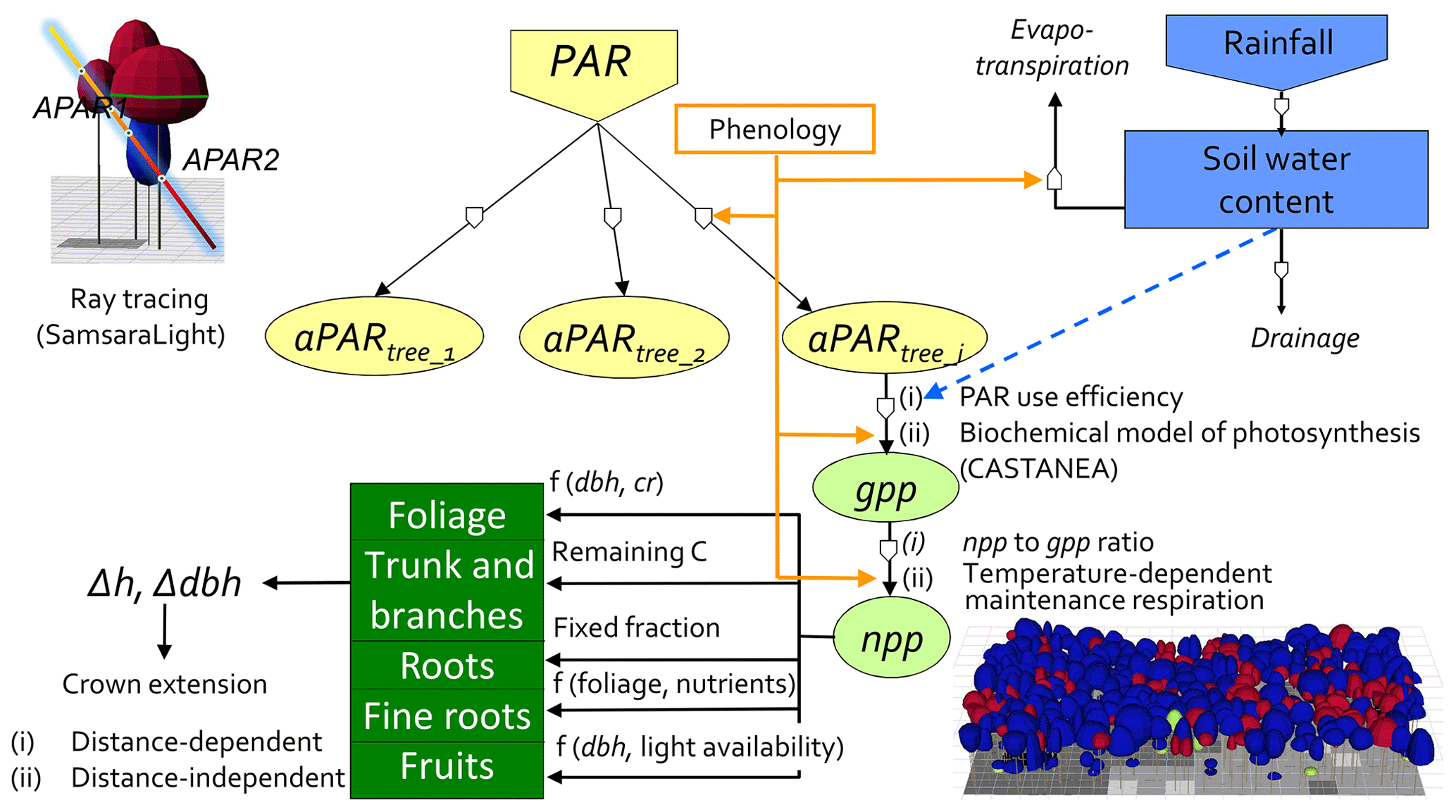
https://www.geosci-model-dev.net/13/905/2020/gmd-13-905-2020-f01

Figure 1Conceptual diagram of the HETEROFOR model. The incident PAR radiation is absorbed by individual trees using a ray-tracing model (SamsaraLight library). Then, the absorbed PAR (aPAR) is converted into gross primary production (gpp) based on the PAR use efficiency concept (first option) or with a biochemical model of photosynthesis (second option). The photosynthesis calculation depends on the soil water potential, which is updated hourly thanks to the water balance module described in detail in de Wergifosse et al. (2019). The net primary production (npp) is obtained using a npp to gpp ratio or by subtracting the growth and maintenance respiration (the latter being temperature dependent). npp is first allocated to foliage using an allometric equation function of tree diameter (dbh) and crown radius (cr). All of these processes (radiation interception, photosynthesis, respiration and evapotranspiration) depend on the foliage development stage, which is determined based on the phenology module. The carbon allocated to fine roots is determined based on a fine root-to-foliage ratio, dependent on the tree nutritional status. Fruit production is calculated with an allometric equation based on dbh and on light availability. The remaining carbon is allocated to structural compartments (roots, trunk and branches) using a fixed proportion for the below-ground part. dbh and height growth (Δdbh and Δh) are deduced from the change in aboveground biomass by deriving and rearranging an allometric equation. Finally, crown extension is predicted with a distance-dependent or distance-independent approach.

Download

2.2 Detailed model description

2.2.1 Initialization

To initialize HETEROFOR, the relative position (x, y, z) and the main dimensions of each tree must be provided, including the following: girth at breast height (gbh; in centimetres), height (h; in metres), height of maximum crown extension (hlce; in metres), height to crown base (hcb; in metres) and crown radii in the four cardinal directions (cr; in metres). During the initialization phase, the biomass of each tree compartment is calculated according to the equations used for carbon allocation (see Sect. 2.2.4. If available, site-specific allometric equations can also be used to calculate initial biomasses of tree compartments. When data on fruit litterfall are available, a file providing the amount of fruit litterfall per year and per tree species can be loaded and used to adapt the allometric equations predicting fruit production at the individual level. When the water balance module is activated, two additional files must be loaded, including a file describing soil horizon properties and another one for the hourly meteorology. Finally, the user must provide the nutrient concentrations of the current leaves (N, P, K, Ca and Mg) for each tree species. These foliar concentrations are then used to estimate the tree nutrient status for each major nutrient. When the tree nutrition and nutrient cycling module is not activated, these concentrations are kept constant throughout the simulation.

2.2.2 Gross primary production

The annual gross primary production of each tree (gpp; in kilograms of C per year) is calculated either based on a PAR use efficiency (PUE) approach (Monteith, 1977) or using the photosynthesis method of the CASTANEA model (Dufrêne et al., 2005). For the first option, the only input needed by the model is the mean monthly global radiation. The second option requires hourly meteorological data and the activation of the water balance calculation. In any case, a series of intermediate variables are needed to calculate gpp.

For the PUE approach, the model uses the solar radiation absorbed by each tree during the vegetation period (aRAD; in megajoules per year); aRAD is then converted in PAR (aPAR; in moles of photons per year) by supposing that 46 % of the solar radiation (RAD) is PAR and 1 MJ is equivalent to 4.55 moles of photons. The diffuse and direct components of aPAR are also considered (aPAR_diff and aPAR_dir; in moles of photons per year). While all of the leaves receive diffuse PAR, only sunlit leaves absorb direct PAR. To estimate the sunlit-leaf proportion (Prop_sl) at the tree level, HETEROFOR uses an adaptation of the classical stand-scale approach based on the Beer–Lambert law (Teh, 2006):

\begin{matrix} (1) & {Prop}_{sl} = \frac{1 - \exp (- k \cdot LAI)}{k}, \end{matrix}

with k, the extinction coefficient, and LAI, the leaf area index (in square metres per square metre).

At the individual scale, the leaf area index is calculated by dividing the tree leaf area (a_leaf; in square metres) by the crown projection area (cpa; in square metres). The value obtained is then multiplied by the light competition index (LCI; in megajoules per megajoule) to account for the shading effect of the neighbouring trees as follows:

\begin{matrix} (2) & {Prop}_{sl} = \frac{1 - \exp (- k \cdot \frac{a_{leaf}}{cpa})}{k} \cdot LCI, \end{matrix}

where LCI is the ratio between the absorbed radiation calculated with and without neighbouring trees in SamsaraLight. LCI ranges from 0 (no light reaching the tree) to 1 (no light competition).

To adapt the PAR use efficiency (PUE) concept at the tree level, we considered a distinct PUE for sunlit (sl) and shaded (sh) leaves and calculated an average PUE weighted as follows:

\begin{matrix} (3) & \begin{aligned} pue = \\ \frac{{aPAR}_{diff} \cdot ({Prop}_{sl} \cdot {PUE}_{sl} + {Prop}_{sh} \cdot {PUE}_{sh}) + {aPAR}_{dir} \cdot {PUE}_{sl}}{aPAR} . \end{aligned} \end{matrix}

This pue value is then used to calculate gpp based on aPAR and a reducer accounting for water stress (red_water) as follows:

\begin{matrix} (4) & gpp = aPAR \cdot pue \cdot {red}_{water} . \end{matrix}

The default value of red_water is 1, but, when the water balance module is activated, it is set to the ratio between the actual and the potential (i.e. considering no soil water limitation) tree transpiration (t_actual and t_pot; in litres per year). This ratio estimates the fraction of the vegetation period during which stomata are partially or totally closed due to a limitation in soil water availability. Since this ratio is always lower or equal to 1, a correction factor is applied to avoid introducing a bias.

\begin{matrix} (5) & {red}_{water} = \frac{t_{actual}}{t_{pot}} \cdot corr . \end{matrix}

gpp can also be estimated using the photosynthesis method of CASTANEA (Dufrêne et al., 2005). This method consists in the biochemical model of Farquhar et al. (1980) analytically coupled with the approach of Ball et al. (1987) that linearly relates stomatal conductance to the product of the carbon assimilation rate by the relative humidity. The slope of this relationship varies between 0 and 1, with the soil water availability characterized in HETEROFOR based on a decreasing exponential function of the mean soil water potential (see eq. 55 in de Wergifosse et al., 2019). The formulation of Ball et al. (1987) was slightly adapted to the tree level by accounting for the influence of tree height. Indeed, leaf water potential increases with leaf height and induces a decrease in stomatal conductance (Ryan and Yoder, 1997; Schäfer et al., 2000). In eq. (55) in de Wergifosse et al. (2019), stomatal conductance is inversely proportional to the height of maximum crown extension.

The photosynthesis routine requires, at an hourly time step, the direct and diffuse PAR absorbed per unit leaf area. The direct PAR is intercepted only by sunlit leaves and is obtained by multiplying the hourly incident PAR (micromoles of photons per square metre per second) by the proportion of direct PAR absorbed by sunlit leaves. For a tree, this proportion is fixed by default for the whole vegetation period and calculated as the ratio between the direct PAR absorbed per unit sunlit-leaf area during the vegetation period (in moles of photons per square metre per year) and the incident PAR accumulated over the same period (in moles of photons per square metre per year). A similar procedure is used for the diffuse absorbed PAR, except that it is related to the total leaf area. When using the detailed version of SamsaraLight, the proportions of direct/diffuse PAR absorbed per unit leaf area change every hour during the day and depending on the phenological stage. The photosynthesis routine of CASTANEA also requires the foliar nitrogen concentration to estimate the maximal carboxylation rate (Dufrêne et al., 2005).

2.2.3 Growth and maintenance respiration

The value of gpp is converted to annual net primary production (npp; in kilograms of C per year) using either a ratio depending on the crown to stem diameter ratio (Eq. 6) or, after subtraction of growth (gr) and maintenance respiration (mr) (Eq. 7), according to the theory of respiration developed by Penning de Vries (1975).

\begin{array}{l} (6) & npp = gpp \cdot r_{npp_gpp} (DdIndex) \\ (7) & npp = gpp - mr - gr \end{array}

Mäkelä and Valentine (2001) showed that the npp to gpp ratio changes with some tree characteristics (tree height and age). Based on simulated gpp and npp reconstructed by using the model in reverse mode (see Sect. 2.2.7), we tested the impact of several variables characterizing tree dimensions and shape (height, dbh, crown radius, crown volume, crown to stem diameter ratio, and aboveground volume or biomass) on the npp to gpp ratio. The best relationship was obtained with the crown to stem diameter ratio (Dd; in metres per metre), which had a negative effect on the npp to gpp ratio. This indicates that the proportion of gpp lost by respiration increases for trees with a large crown. Unfortunately, the crown to stem diameter ratio not only varies with the tree shape reflecting past competition conditions but also changes during the course of the tree development for some tree species. Therefore, we standardized it to remove the size effect in order to obtain an index (DdIndex) that only characterizes the tree shape. This index is particularly useful in accounting for the large differences in the oak crown extensions according to the silvicultural system (large crowns in former coppices with standards vs. narrow crowns in dense high forests).

\begin{matrix} (8) & r_{npp_gpp} = α + β \cdot DdIndex, \end{matrix}

where α and β are parameters and DdIndex is defined as

\begin{matrix} (9) & DdIndex = \frac{Dd}{{Dd}_{pred}}, \end{matrix}

with Dd, the crown to stem diameter ratio determined from the tree mean crown radius (cr_mean; in metres) and diameter at breast height (dbh; in metres), and Dd_pred, the crown to stem diameter ratio predicted based on the girth at breast height (gbh; in centimetres):

\begin{matrix} (10) & {Dd}_{pred} = α + β \cdot g b h + γ \cdot \frac{1}{gbh} + δ \cdot \frac{1}{{gbh}^{2}} . \end{matrix}

In Eq. (7), maintenance respiration is calculated for each tree by summing the maintenance respiration of each compartment, which is estimated from the nitrogen content of its living biomass, and considering a Q₁₀ function for the temperature dependency. During daytime, the inhibition of foliage respiration by light is taken into account by considering that this inhibition reduces respiration by 62 % (Villar et al., 1995).

\begin{matrix} (11) & mr = \sum_{comp.} (b_{comp.} \cdot f_{living} \cdot [N] \cdot R_{T_{ref}} \cdot Q_{10_comp.}^{\frac{T - T_{ref}}{10}}), \end{matrix}

with b_comp., the tree compartment biomass (kilograms of organic matter), f_living, the fraction of living biomass, [N], the nitrogen concentration (in grams per kilogram), $R_{T_{ref}}$ , the maintenance respiration per gram of N at the reference temperature (15 ^∘C), and T, the air temperature for aboveground tree compartments or the soil horizon temperature for roots (see Appendix A). Root maintenance respiration is estimated for each soil horizon separately.

The fraction of living biomass is fixed to 1 for leaves and fine roots or equals the proportion of sapwood for the structural tree compartments. The sapwood proportion is derived from the sapwood area (a_sapwood; in square centimetres), which is determined based on an empirical function of the tree compartment diameter (∅_comp.; in centimetres) as follows:

\begin{matrix} (12) & a_{sapwood} = a + b \cdot \emptyset_{comp.} + c \cdot \emptyset_{comp.}^{2} . \end{matrix}

Growth respiration (gr) is the sum of the tree compartment growth respirations, which are proportional to their biomass increments (see Sect. 2.2.4).

\begin{matrix} (13) & gr = \sum_{comp.} (R_{gr} \cdot Δ b_{comp.}), \end{matrix}

where R_gr is the growth respiration per unit biomass increment (in kilograms of C per kilogram of C).

2.2.4 Carbon allocation and dimensional growth

For each tree, the npp and the carbon retranslocated from leaves and roots (rt_leaf and rt_fine root; in kilograms of C per year) are distributed among the various tree compartments at the end of the year. rt_leaf and rt_fine root are determined as follows:

\begin{matrix} (14) & \begin{aligned} {rt}_{leaf or fine root} = \\ b_{leaf or fine root} \cdot δ_{leaf or fine root} \cdot {rtr}_{leaf or fine root}, \end{aligned} \end{matrix}

where b_leaf and b_fine root are the tree leaf and fine root biomasses (in kilograms of C), δ_leaf and δ_fine root are the leaf and fine root turnover rates (in kilograms of C per kilogram of C per year), and rtr_leaf and rtr_fine root are the leaf and fine root retranslocation rates (in kilograms of C per kilogram of C).

b_leaf is estimated with an allometric equation based on the stem diameter at breast height (dbh; in centimetres) and on the crown to stem diameter ratio (Dd),

\begin{matrix} (15) & b_{leaf} = α \cdot {dbh}^{β} \cdot {Dd}^{γ} . \end{matrix}

b_fine root is deduced from the leaf biomass using the fine root to leaf ratio (r_{fine root_leaf}) as follows:

\begin{matrix} (16) & b_{fine root} = b_{leaf} \cdot r_{fine root_leaf} . \end{matrix}

r_{fine root_leaf} takes a value between a minimum (r_{fine root_leaf_min}) and maximum (r_{fine root_leaf_max}) ratio, depending on the tree nutritional status, in accordance with the concept of functional balance (Mäkela, 1986). This means that a higher ratio (more carbon allocation to fine roots) is used when tree suffers from nutrient deficiency. For each nutrient, a candidate ratio is obtained based on a linear relationship depending on the nutritional status. The ratio increases when the nutritional status deteriorates, and this effect is more pronounced for nitrogen (N), with nitrogen (N) > phosphorus (P) > potassium (K) > magnesium (Mg) > calcium (Ca). Among the candidate ratios, the maximum is retained in order to account for the fact that the most limiting nutrient has the dominant effect. For each nutrient, the nutritional status is bounded between 0 and 1 and calculated based on the foliar concentrations (provided in the inventory file) and the optimum and deficiency thresholds (Mellert and Göttlein, 2012).

\begin{matrix} (17) & Status (Nutrient) = \frac{[Foliar Nutrient] - Deficiency}{Optimum-Deficiency} . \end{matrix}

The leaf and fine root litter amounts (s_leaf and s_fine root; in kilograms of C per year) are estimated based on the turnover rate taking into account the retranslocation as follows:

\begin{matrix} (18) & \begin{aligned} s_{leaf or fine root} = \\ b_{leaf or fine root} \cdot δ_{leaf or fine root} \cdot (1 - {rt}_{leaf or fine root}) . \end{aligned} \end{matrix}

Allocation priority is given to leaves and fine roots. The carbon allocated to leaves corresponds to the annual leaf production (p_leaf; in kilograms of C per year), which is equal to the fallen leaf biomass of the previous year plus the leaf biomass change (Δb_leaf; in kilograms of C per year),

\begin{matrix} (19) & p_{leaf} = b_{{leaf}_{t - 1}} \cdot δ_{leaf} + Δ b_{leaf}, \end{matrix}

where Δb_leaf is determined by

\begin{matrix} (20) & Δ b_{leaf} = b_{{leaf}_{t}} - b_{{leaf}_{t - 1}}, \end{matrix}

where $b_{{leaf}_{t - 1}}$ and $b_{{leaf}_{t}}$ are the tree leaf biomasses corresponding to the previous and the current years, respectively.

The fine root production is then estimated according to the same logic.

\begin{matrix} (21) & p_{fine root} = b_{{fine root}_{t - 1}} \cdot δ_{fr} + Δ b_{fr}, \end{matrix}

where $b_{{fine root}_{t - 1}}$ is provided by Eq. (16).

When the carbon allocated to leaves and fine roots is higher than the npp plus the retranslocated carbon (suppressed trees with low gpp and npp for their size), the leaf and fine root productions are recalculated so that they do not exceed 90 % of the available carbon.

Then, the fruit production (p_fruit; in kilograms of C per year) is estimated with an allometric equation similar to Eq. (15) and is considered directly proportional to the light competition index since fructification is known to be favoured when tree crowns are exposed to the sun (Greene et al., 2002; Davi et al., 2016). A threshold dbh (dbh_threshold; in centimetres) is fixed, below which no fruit production occurs.

\begin{matrix} (22) & p_{fruit} = α \cdot LCI \cdot (dbh - {dbh}_{threshold})^{β} \end{matrix}

In this equation, the parameter α takes a default value or is adapted based on the fruit production of the year (when the file with the amount of fruit litterfall per year and per tree species is loaded).

Part of the carbon is also used to compensate for branch and root mortality. The branch mortality (s_branch; in kilograms of C per year) is described with an equation of the same form as Eq. (15), while the structural root mortality (s_root; in kilograms of C per year) is obtained using a turnover rate similar to that of the branches.

After subtracting the leaf, fine root and fruit productions and the root and branch senescence, the remaining carbon is allocated to structural tree compartment growth:

\begin{matrix} (23) & Δ b_{structural} = npp + rt - p_{leaf} - p_{fine root} - p_{fruit} - s_{branch} - s_{root} . \end{matrix}

At this stage, the remaining carbon is partitioned between the above- and below-ground parts of the tree according to a fixed root-to-shoot ratio (r_{root_shoot}) as follows:

\begin{array}{l} (24) & Δ b_{structural_above} = \frac{Δ b_{structural}}{(1 + r_{root_shoot})} \\ (25) & Δ b_{structural_below} = Δ b_{structural} - Δ b_{structural_above} . \end{array}

The increment in aboveground structural biomass is then used to determine the combined increment in dbh and total height (h; in metres) based on an allometric equation used to predict aboveground woody biomass (Genet et al., 2011; Hounzandji et al., 2015),

\begin{matrix} (26) & b_{structural_above} = α + β ({dbh}^{2} \cdot h)^{γ} . \end{matrix}

Deriving this equation and rearranging terms gives

\begin{array}{l} (27) & Δ b_{structural_above} = β γ ({dbh}^{2} \cdot h)^{γ - 1} Δ ({dbh}^{2} \cdot h) \\ (28) & Δ ({dbh}^{2} \cdot h) = \frac{Δ b_{structural_above}}{β γ ({dbh}^{2} \cdot h)^{γ - 1}} . \end{array}

The development of the left term provides

\begin{matrix} (29) & Δ ({dbh}^{2} \cdot h) = (dbh + Δ dbh)^{2} \cdot (h + Δ h) - {dbh}^{2} \cdot h, \end{matrix}

which can be further developed (see Appendix B for details) to isolate Δh:

\begin{matrix} (30) & Δ h ≅ \frac{Δ ({dbh}^{2} \cdot h)}{{dbh}^{2}} - \frac{h \cdot Δ {dbh}^{2}}{{dbh}^{2}} \end{matrix}

From Eq. (30), we know that the height increment can be expressed as a function of $\frac{Δ ({dbh}^{2} \cdot h)}{{dbh}^{2}}$ . In the following, we refer to it as the height growth potential (Δh_pot) since it corresponds to the height increment if all of the remaining carbon was allocated to height growth. Contrary to the other term of Eq. (30) $(\frac{h \cdot Δ {dbh}^{2}}{{dbh}^{2}})$ , which is unknown, this height growth potential can be evaluated at this step by dividing the result of Eq. (28) by dbh². However, depending on the level of competition for light and on the tree size, only part of this height growth potential will be effectively realized for the height increment. For each tree species, an empirical relationship, predicting height growth from the height growth potential, the light competition index and the tree size (dbh or height), was therefore fitted based on successive inventory data (see Appendix E).

\begin{matrix} (31) & \begin{aligned} Δ h = & a + b \cdot dbh + c \cdot h + d \cdot LCI + e \cdot Δ h_{pot} \\ + f \cdot {(Δ h_{pot})}^{2} + g \cdot {(Δ h_{pot})}^{3} \end{aligned} \end{matrix}

The dbh increment is then determined by rearranging Eq. (29) as follows:

\begin{matrix} (32) & Δ dbh = \sqrt{\frac{Δ ({dbh}^{2} \cdot h) + {dbh}^{2} \cdot h}{(h + Δ h)}} - dbh . \end{matrix}

The increments in root, stem and branch biomasses are obtained as follows:

\begin{matrix} (33) & Δ b_{root} = r_{root_shoot} \cdot Δ b_{structural_above} \\ (34) & \begin{aligned} Δ b_{stem} = \\ f \cdot ρ \cdot ({(dbh + Δ dbh)}^{2} \cdot (h_{del} + Δ h_{del}) - {dbh}^{2} \cdot h_{del}) \end{aligned} \\ (35) & Δ b_{branch} = Δ b_{structural_above} - Δ b_{stem}, \end{matrix}

where f is the form coefficient (in cubic metres per cubic metre), ρ is the stem volumetric mass (in kilograms of C per cubic metre) and h_del is the Delevoy height (in metres) corresponding to the height at which stem diameter is half the diameter at breast height (see Appendix C).

The branch and root biomasses are then distributed in three categories, defined based on the diameter, which are as follows: small branches/roots < 4 cm, medium branches/roots between 4 and 7 cm and coarse branches/roots > 7 cm. The proportions of small, medium and coarse branches/roots are determined based on equations of the same form as those presented in Hounzandji et al. (2015) for oak branches. Until we can adjust these equations on appropriate data sets, the parameters of Hounzandji et al. (2015) are also used for beech branches and for oak and beech roots. The distribution in the root categories has no impact on the functioning of the model since this information is not used elsewhere. This is just a model output that the user can ignore or consider as a whole.

2.2.5 Crown extension

Depending on whether the competition with the neighbouring trees is taken into account or not, the crown dynamics can be described by two different approaches. When local competition is not considered (distance-independent approach), changes in crown dimensions are derived from dbh or height increment based on the following empirical relationships:

\begin{array}{l} (36) & Δ hlce = hlce % \cdot Δ h \\ (37) & Δ hcb = hcb % \cdot Δ h \\ (38) & Δ cr = {Dd}_{pred} \cdot \frac{Δ dbh}{200}, \end{array}

where hcb% and hlce% are the proportions of the total height corresponding to the height to crown base (hcb; in metres) and to the height of largest crown extension (hlce; in metres), respectively; Δcr is the change in crown radius (in metres) whatever the direction; Dd_pred is the crown to stem diameter ratio estimated by Eq. (10).

Alternatively, the changes in crown dimensions can be described based on the competition with the neighbouring trees (distance-dependent approach). The space around a target tree is divided into four sectors according to the four cardinal directions (north between 315 and 45^∘, east between 45 and 135^∘, south between 135 and 225^∘, and west between 225 and 315^∘). In each sector, the tree that is the closest to the target tree is retained as a competitor if its height is higher than the hcb of the target tree. Beyond a certain distance (i.e. 2 times the maximal crown radius of 10 m), no competitor is considered. For each main direction, the model calculates an hlce at equilibrium (hlce_eq; in metres) for the target tree. This hlce at equilibrium is located between a minimum (hcb; in metres) and a maximum (hlce_max; in metres). hlce_max is obtained by determining the higher intersection between the potential crowns of the target tree and the competitor. The potential crown of a tree is the crown that this tree would have had in absence of competition and is considered as having the shape of a half-ellipsoid, centred on the tree trunk and with the semi-axis lengths equal to the tree potential crown radius (cr_pot; in metres; see below) and to the crown length (h−hcb). hlce_eq is positioned between the minimum and the maximum values according to the competition intensity, estimated based on the target tree and the competitor heights (h_target and h_comp; in metres), as well as the hcb of the target tree (Appendix D).

\begin{matrix} (39) & \begin{aligned} {hlce}_{eq} = \\ hcb + ({hlce}_{max} - hcb) \cdot max (0, min (1, \frac{h_{comp} - hcb}{h_{target} - hcb})) \end{aligned} \end{matrix}

The four values of hlce_eq are then averaged (hlce_{eq_mean}).

Finally, the change in hlce is determined as follows:
if hlce<hlce_{eq_mean},

\begin{matrix} (40) & Δ hlce = min (Δ {hlce}_{max}, {hlce}_{eq_mean} - hlce) \end{matrix}

else,

\begin{matrix} (41) & Δ hlce = max (- Δ {hlce}_{max}, {hlce}_{eq_mean} - h l c e), \end{matrix}

where Δhlce_max is the maximum change in hlce allowed by the model.

The change in hcb is obtained with the same logic.
If hcb<hcb_{eq_mean},

\begin{matrix} (42) & Δ hcb = min (Δ {hcb}_{max}, {hcb}_{eq_mean} - hcb), \end{matrix}

else,

\begin{matrix} (43) & Δ hcb = max (- Δ {hcb}_{max}, {hcb}_{eq_mean} - hcb), \end{matrix}

where hcb_{eq_mean} is the hcb estimated from the tree height based on hcb% (Eq. 37).

The changes in the four crown radii are calculated based on crown radii at equilibrium (cr_eq; in metres), which are estimated by considering the competitive strength of the target and neighbouring trees. For a given direction, cr_eq is calculated based on the potential (free-growth) crown radius of the target tree (cr_{pot_target}; in metres) and its competitor (cr_{pot_comp}; in metres), the distance between the two trees (d; in metres), and the crown overlap ratio (r_overlap; in metres per metre) as follows:

\begin{matrix} (44) & {cr}_{eq} = \frac{{cr}_{pot_target}}{{cr}_{pot_target} + {cr}_{pot_comp}} \cdot d \cdot r_{overlap_target} . \end{matrix}

The potential crown radius (cr_pot) of a tree if determined by

\begin{matrix} (45) & {cr}_{pot} = \frac{dbh}{200} \cdot {Dd}_{pred} \cdot sh, \end{matrix}

where Dd_pred is the crown to stem diameter ratio estimated by Eq. (10), and sh is a coefficient allowing a shift from the mean to the maximum Dd_pred.

The crown overlap ratio is estimated by considering neighbouring trees of the same species two by two and then calculating the ratio between the sum of their crown radii and the distance between the corresponding tree stems. This overlap ratio accounts for the capacity of a tree species to penetrate in neighbouring crowns.

The change in crown radius is then determined for each direction as follows:
if cr<cr_eq,

\begin{matrix} (46) & Δ cr = min (Δ {cr}_{max} {cr}_{eq} - cr), \end{matrix}

else,

\begin{matrix} (47) & Δ cr = max (- Δ {cr}_{max} {cr}_{eq} - cr), \end{matrix}

where Δcr_min and Δcr_max are respectively the minimum and the maximum change in cr allowed by the model. They are obtained in a similar way as cr_pot, with

\begin{matrix} (48) & Δ {cr}_{max} = \frac{Δ dbh}{200} \cdot Dd \cdot sh . \end{matrix}

2.2.6 Tree harvesting and mortality

During the simulation, thinning can be achieved at each annual step by (i) selecting the trees from a list or a map or according to tree characteristics (tree species, age, dbh, height, etc.), (ii) defining the number of trees to be thinned per diameter class using an interactive histogram, or (iii) loading a file listing the trees that must be thinned. In addition, the thinning methods developed for GYMNOS and QUERGUS are compatible with HETEROFOR. They allow one to reach a target basal area, density or relative density index by thinning from below or from above or by creating gaps (Ligot et al., 2014).

When the npp of a tree is not sufficient to ensure a normal leaf and fine root development (for suppressed trees and/or after a severe drought), the leaf biomass is reduced and induces a defoliation, which is estimated as follows:

\begin{matrix} (49) & Def = \frac{b_{leaf} - b_{leaf_corr}}{b_{leaf}} \cdot 100, \end{matrix}

where b_leaf and b_{leaf_corr} are, respectively, the leaf biomass estimated with Eq. (15) and the leaf biomass corrected to match the available carbon (see Sect. 2.2.4).

Tree mortality occurs when trees reach a defoliation of 90 %, considering that a tree with less than 10 % of its leaves is in an advanced stage of decline and is unlikely to recover (Manion, 1981). Hence, HETEROFOR takes into account the mortality resulting from carbon starvation due to light competition and/or water stress (stomatal closure).

2.2.7 Growth reconstruction

HETEROFOR was adapted to allow the user to run it in reverse mode by starting from the known increments in dbh and h to reconstruct an individual npp using exactly the same parameters and equations as in the normal mode. To achieve a reconstruction, an inventory file with tree measurements must be loaded to create the initial step. From this initial step, the reconstruction tools can be launched and require another inventory file with tree measurements achieved one or several years later. Based on these two inventories, HETEROFOR calculates the mean dbh and h increments for each tree and uses the model equations to reconstruct each step and evaluate among other individual npp's. The npp is obtained by rearranging Eq. (23), in which the carbon allocated to the structural biomass is calculated from the dbh and h increments using Eqs. (27), (25) and (24). The carbon allocated to leaf, fine root and fruit production is determined, respectively, with Eqs. (19), (21) and (22), while the amount retranslocated from leaves and roots before senescence is evaluated with Eq. (14). Finally, the terms of Eq. (23) accounting for the leaf and fine root litter were determined with Eq. (18). In addition to two stand inventories, the reconstruction tool also requires a file listing the trees which were cut or died between the two inventory dates and the last year during which they were present in the stand.

2.3 Input variables and parameter setting for a case study

The model was tested in three stands that contrast in structure and species composition. These stands were located close to each other (< 1 km) on the same tableland (300 m elevation) in the western part of the Belgian Ardennes at Baileux (50^∘01^′ N, 4^∘24^′ E). The average annual rainfall is slightly above 1000 mm, and the mean annual temperature is 8 ^∘C. The forest (60 ha) consists of sessile oaks (Quercus petraea Liebl.) and European beeches (Fagus sylvatica L.) and lies on acid brown earth soil (Luvisol according to the FAO soil taxonomy) with a moder humus and an A_hB_wC profile. The soil has been developed on a loamy and stony solifluction sheet in which weathering products of the bedrock (Lower Devonian: sandstone and schist) were mixed with added periglacial loess.

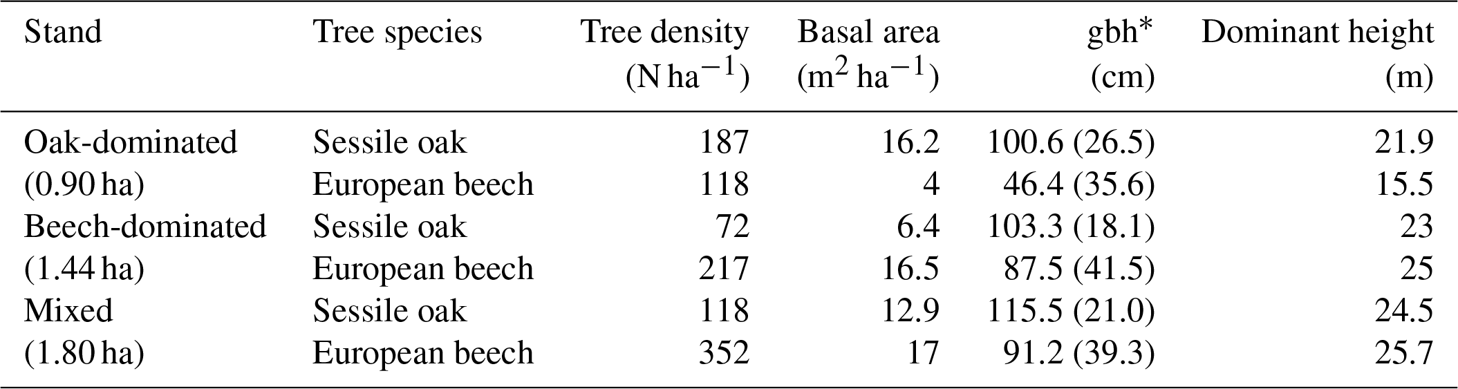
Table 1Stand characteristics for the main tree species derived from stand inventories in 2001. Standard deviation is provided in parentheses.

^* Girth at breast height.

Download Print Version | Download XLSX

By the end of the 19th century, the Baileux forest was probably an oak coppice with a few standards. Taking advantage of the massive oak regeneration in the 1880s, the forest developed progressively into a high forest and was then invaded by beeches. In 2001, the area was covered by even-aged oak trees and heterogeneously sized beech trees. At that time, three experimental plots were installed at the Baileux site in order to study the impact of tree species mixing on ecosystem functioning (Jonard et al., 2006, 2007, 2008; André et al., 2008a, b, 2010, 2011); two plots were located in stands dominated by either sessile oak or beech, and the third one was a mixture of both species (Table 1). In each plot, all trees with a circumference higher than 15 cm were mapped (coordinates) and measured (stem circumference at a height of 1.3 m, total tree height, height of largest crown extension, height to crown base and crown diameters in two directions) at the end of the years 2001 and 2011.

Meteorological data were monitored with an automatic meteorological station located in an open field that is 300 m away from the forest site. Soil horizon properties were characterized based on the soil profile description and the measurements carried out by Jonard et al. (2011).

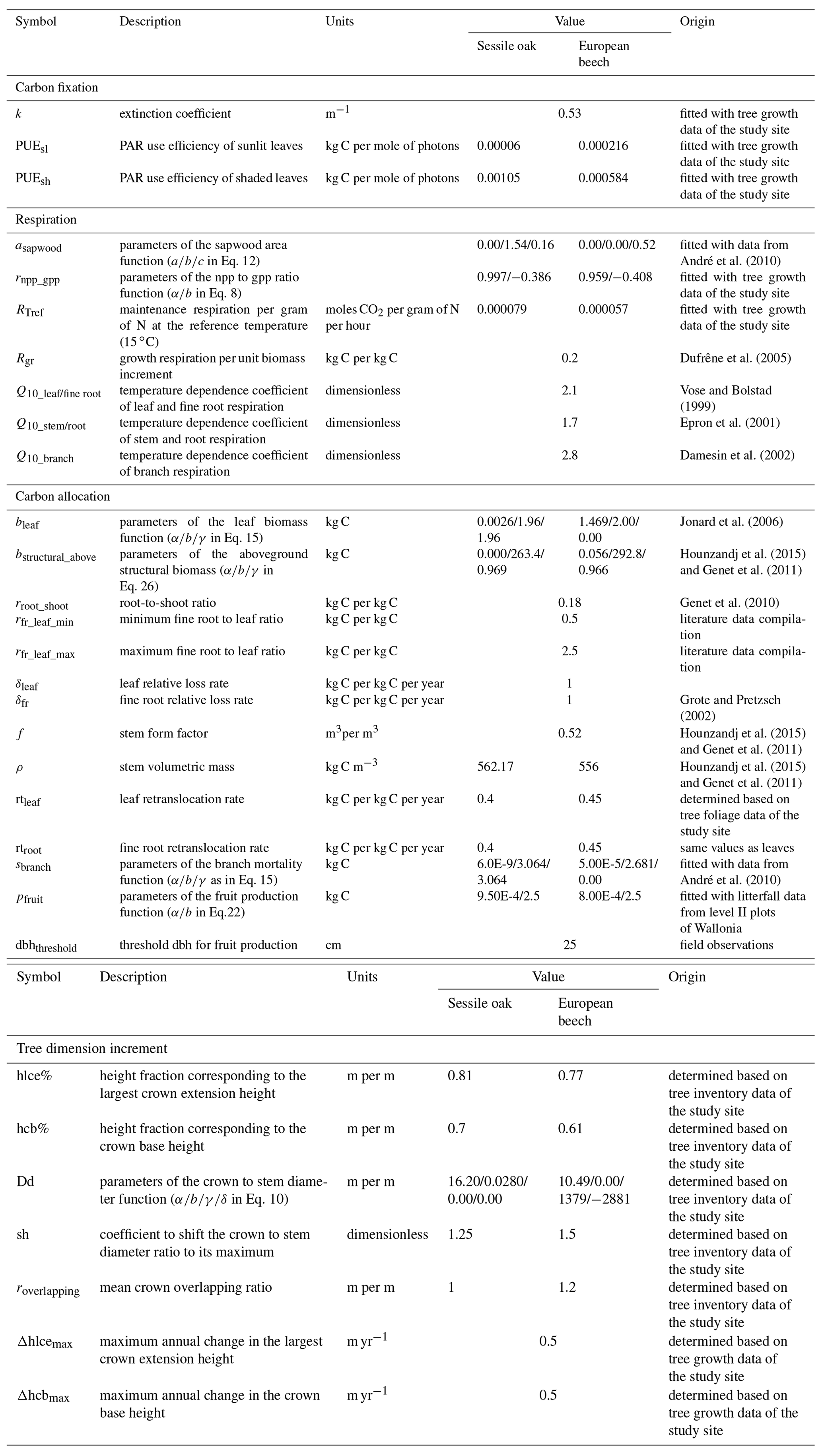
To run the simulations, the values of some model parameters were taken directly from the literature. Other parameters involved in empirical relationships were fitted with either data from previous studies or unpublished monitoring data collected in the study site or in the International Co-operative Programme on Assessment and Monitoring of Air Pollution Effects on Forests (ICP Forests) level II plots of Wallonia (Table 2). Potential explanatory variables in Eq. (31) used to estimate height growth were selected by applying a stepwise forward selection procedure based on the Bayesian information criterion (BIC). A multivariate model was then adjusted with the selected variables (Appendix E). The parameters of the npp to gpp ratio relationship, the maintenance respiration per gram of nitrogen at 15 ^∘C, and the PAR use efficiency of sunlit and shaded leaves were adjusted with the nonlinear minimization (nlm) function in R (R Core Team, 2013) based on observed basal area increments (BAIs) using the maximum likelihood approach. This calibration was completed only based on the data of the mixed stand, while the model performances were evaluated with observations from the three stands of the Baileux site.

Table 2Description of model parameters for sessile oak and European beech and origin of their value.

Download XLSX

All the simulations carried out in this study were run with the default option for modelling phenology and water balance (de Wergifosse et al., 2019). In addition, since the tree nutrition and nutrient cycling module was not activated, the tree nutrient status remained constant during the simulations.

2.4 Statistical evaluation of model predictions

The quality of the model was evaluated for various combinations of model options (i.e. photosynthesis model of CASTANEA vs. PUE, npp to gpp ratio vs. temperature-dependent maintenance respiration and distance-dependent vs. independent crown extension) by comparing predicted and observed BAIs using several statistical indices and tests such as the normalized average error, the P value of the paired t test, the regression test, the root mean square error and the Pearson's correlation (Janssen and Heuberger, 1995). For the regression test, the Deming fitting procedure (mcreg function of the mcr package in R) was retained to account for the errors in both the observations and the predictions. For all of the simulations, the water balance module was activated. Some option combinations were therefore not tested, such as the PUE approach without activating the water balance.

The model quality was also evaluated based on its ability to reconstruct the size–growth relationships for the sessile oak and European beech in the three stands in Baileux. The observed and predicted BAIs of the trees (calculated for the 2001–2011 period) were related to their girth at the beginning of the assessment period. A segmented regression was then applied to observations and predictions to determine the girth threshold beyond which the basal area increment (BAI) linearly increases with girth and to estimate the slope of the linear relationship between the BAI and initial girth. The heteroscedasticity of the residuals was accounted for by modelling their standard deviation with a power function of the initial girth. The fitting was carried out using the nlm function in R.

2.5 Simulation experiment

To assess how the tree biomass production and its allocation to the different tree compartments were affected by climate conditions and management in the model, we simulated the development of the mixed stand during a dry (2003, with P=948 mm and T_air=9.88 ^∘C), a normal (2005, with P=1027 mm and T_air=9.67 ^∘C) and a wet year (2012, with P=1117 mm and T_air=9.37 ^∘C), and we repeated these simulations after thinning this stand by reducing its basal area by 25 %. The biomass production and its allocation were assessed at the stand level as well as at the tree level for seven cohorts (four beech cohorts and three oak cohorts), defined based on the tree species and on the girth-class distribution. For this first simulation experiment, we used the following options: photosynthesis model of CASTANEA, npp to gpp ratio and distance-independent crown extension.

A second simulation experiment was performed to illustrate how the model can be used to predict climate change impacts on the functioning of the forest ecosystem. The growth dynamics in the mixed stand in Baileux was simulated according to three IPCC climate scenarios using the following options: photosynthesis model of CASTANEA, npp to gpp ratio and distance-independent crown extension. The climate scenarios retained for this study were obtained from the global circulation model CNRM-CM5 (Voldoire et al., 2013) based on the representative concentration pathways (RCPs) for atmospheric greenhouse gases described in the Fifth Assessment Report of the Intergovernmental Panel on Climate Change (Collin et al., 2013). The representative concentration pathways (RCP2.6, RCP4.5 and RCP8.5) are characterized by the radiative forcing in the year 2100 relative to preindustrial levels (+2.6, +4.5 and +8.5 W m⁻²). The CNRM-CM5 describes the earth system climate using variables such as air temperature and precipitation on a low-resolution grid (1.4^∘ in latitude and longitude). Although reliable for estimating global warming, such a model fails to capture the local climate variations. Therefore, these climate projections were downscaled by the Royal Meteorological Institute of Belgium (RMI), using the regional climate model ALARO-0 (Giot et al., 2016). The meteorological files that were received from RMI are hourly values of the longwave and shortwave radiation, air temperature, surface temperature, rainfall, specific humidity, zonal and meridional wind speeds and atmospheric pressure with a 4 km spatial resolution. Specific humidity was converted into relative humidity using the Tetens formula (Tetens, 1930). For a reference period (1976–2005), we compared the models predictions with observed meteorological data and detected some biases, especially for precipitation (overestimation of 27 %). To correct these biases, we applied correction factors depending on the month (Maraun and Widmann, 2018). An additive correction factor was used for the bounded variables (radiation, precipitation, relative humidity and wind speed), and a multiplicative was used for the other variables (air and surface temperatures).

For the simulations, two 24-year periods (100 years apart) were considered. The period from 1976 to 1999 served as a historical reference, while the rest of the simulations based on climate projections were conducted for the 2076–2099 period. The simulations were performed by either keeping the CO₂ concentration of the atmosphere constant (i.e. 380 ppm) or allowing it to vary yearly according to the climate scenarios. Each simulation started with the same initial stand (mixed stand in Baileux in 2001) and lasted 24 years; a thinning operation (25 % in basal area) was carried out in 1978 or 2078 and in 1990 or 2090 (12-year cutting cycle). The mean basal area increments obtained with the various climate scenarios were compared using the Tukey multiple comparison test.

Table 3Statistical evaluation of predicted basal area increments (vs. observations) for various combinations of model options using normalized average error (NAE), paired t test, regression test, root mean square error (RMSE) or Pearson's correlation (Pearson's r). Standard deviation or confidence intervals are provided in parentheses.

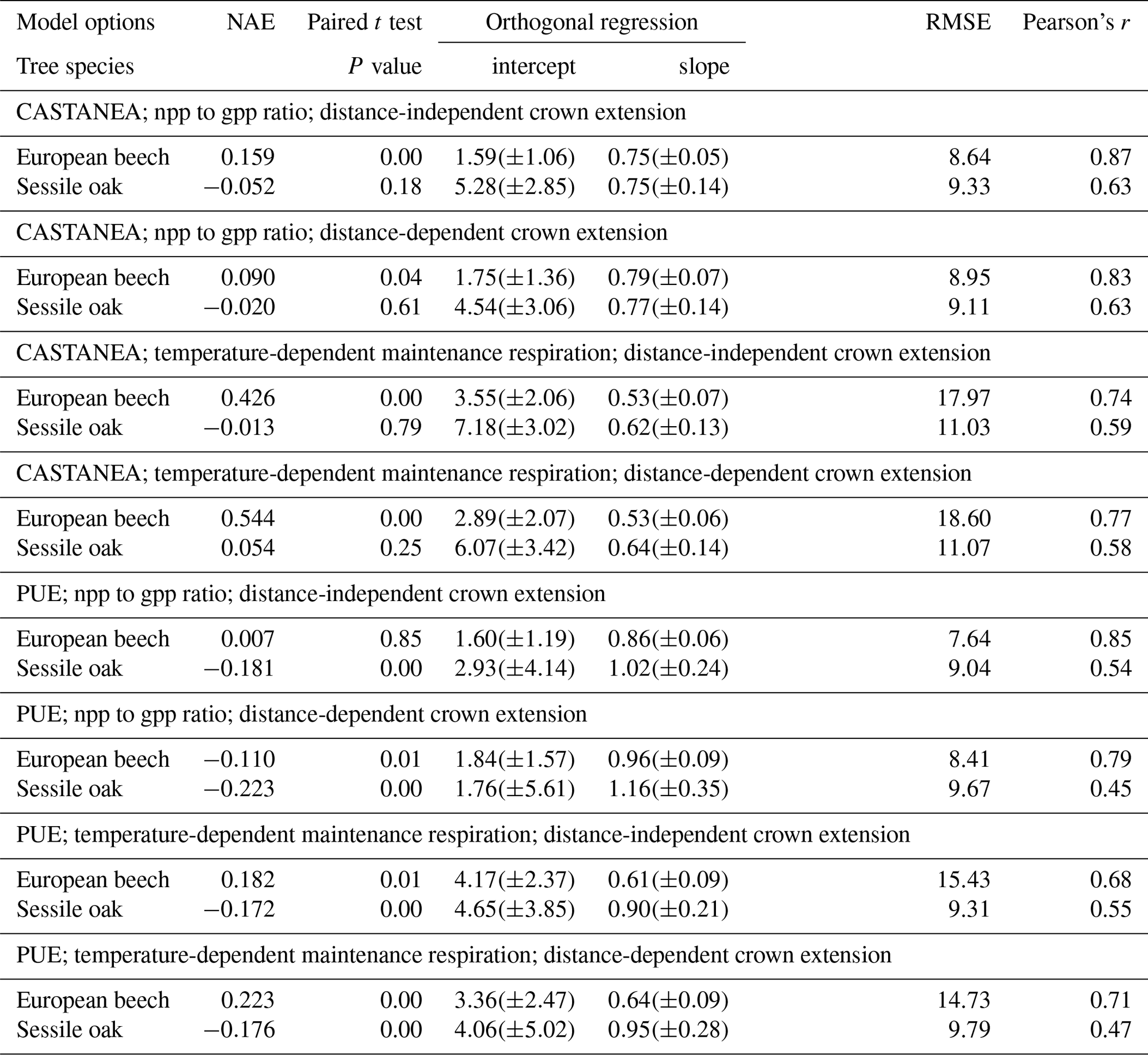
Download Print Version | Download XLSX

https://www.geosci-model-dev.net/13/905/2020/gmd-13-905-2020-f02

Figure 2Relationship between the individual npp reconstructed based on successive stand inventories (2001 and 2011) and the gpp predicted with the process-based option (photosynthesis method of CASTANEA) for the three stands. Values in parentheses are 95 % confidence intervals for the intercept and the slope in the equations. The Pearson's correlation between npp and gpp is indicated on the graph.

Download

3 Results

3.1 Reconstructed npp vs. predicted gpp

Based on two successive stand inventories (2001 and 2011) and using HETEROFOR in reverse mode (see Sect. 2.2.7), the individual npp was reconstructed and related to the gpp predicted with the photosynthesis method of CASTANEA. The linear relationship between npp and gpp explained 79 % and 83 % of the variability in sessile oaks and European beeches, respectively (Fig. 2). The intercept was positive and just significantly different from 0 but did not differ between the two trees species. The slope of the relationship was higher for the sessile oak (0.50) than for European beech (0.40).

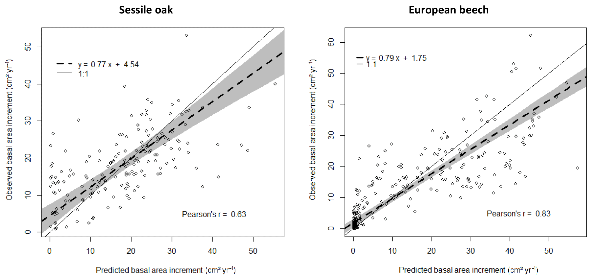
https://www.geosci-model-dev.net/13/905/2020/gmd-13-905-2020-f03

Figure 3Comparison of observed and predicted basal area increments (BAIs) for the simulation with the photosynthesis method of CASTANEA, the npp to gpp ratio approach to account for tree respiration and the distance-dependent crown extension (see Table 3). The dashed line represents the Deming regression between observations and predictions, with the shaded area indicating the 95 % confidence interval and the solid line the 1 : 1 relationship.

Download

https://www.geosci-model-dev.net/13/905/2020/gmd-13-905-2020-f04

Figure 4Reconstruction of the size–growth relationships for sessile oak and European beech in the three stands using the photosynthesis method of CASTANEA, the npp to gpp ratio approach to account for tree respiration and the distance-dependent crown extension. The predicted relationships between the individual BAI (calculated for the 2001–2011 period) and the initial girth are compared with observed ones. The solid and dashed lines represent the segmented regression applied, respectively, to observations and predictions to determine the girth threshold beyond which radial growth linearly increases with girth and to estimate the slope of the linear relationship between BAI and initial girth. The 95 % confidence intervals for the intercept and the slope are provided as well as the R² of the model. No relationship was fitted for the European beech in the oak-dominated stand given the lack of data.

Download

3.2 Model performance in predicting individual basal area increment (BAI)

HETEROFOR was run with different combinations of options for describing photosynthesis (biochemical model of CASTANEA vs. PUE), respiration (npp to gpp ratio vs. temperature-dependent maintenance respiration) and crown extension (distance-dependent vs. distance-independent). The predictions carried out using the photosynthesis routine of CASTANEA were generally slightly better correlated to the observations than those obtained with the PUE approach, which however displayed somewhat lower RMSE (Table 3). For both of the photosynthesis calculation options, the use of the maintenance respiration routine provided less accurate predictions (higher NAE and RMSE and lower Pearson's r) than the npp to gpp ratio approach, and the degradation of the model performance due to the maintenance respiration option was more marked for the European beech than for the sessile oak (Table 3). The option for describing crown extension had little effect on prediction quality. Depending on the criterion considered, the options selected for calculating photosynthesis and respiration and the tree species, the distance-independent approach was sometimes the best but not in all cases (Table 3).

For the simulations using the CASTANEA photosynthesis, we retained the npp to gpp approach and the distance-dependent crown extension as the best combination of options since the associated predictions were on average not biased for oak and only slightly biased for beech (Table 3). For this combination of options, the regression of the observed BAIs on the predictions showed however a slight underestimation of the low BAIs and a small overestimation of the high BAIs, which were more pronounced for the European beech than for the sessile oak (Fig. 3). For the PUE method, the npp to gpp ratio and the distance-independent crown extension provided the most accurate predictions (Table 3).

3.3 Reconstructing size–growth relationships

The size–growth relationships were very similar between observations and predictions for the mixed stand on which the model was calibrated (Fig. 4). For the European beech in the beech-dominated stand, the predicted increase in BAI with the initial girth was steeper than the observed increase, revealing a slight overestimation of the tree growth (Fig. 4). The proportion of the BAI variance explained by the size–growth relationship (R²) was higher for the European beech than for the sessile oak for both observations and predictions (Fig. 4).

3.4 Simulation of climate change impact on tree growth

In the first simulation experiment, the effect of thinning was much more pronounced on the smallest trees than on the biggest ones (Fig. 5). The smallest beech cohort (girth of 0 to 61 cm) almost doubled their annual biomass production after the thinning (+85 %), while the thinning impact on the biggest oak and beech trees was hardly noticeable (+4 % and +2 %, respectively). When looking at the different tree compartments, one may notice that the thinning effect was more pronounced on the structural compartments, i.e. roots, stem and branches (+52 %), than on the functional ones, i.e. fine roots, leaves and fruits (+22 %). While thinning increased the individual biomass production, it decreased the biomass production at the stand level (−15 %).

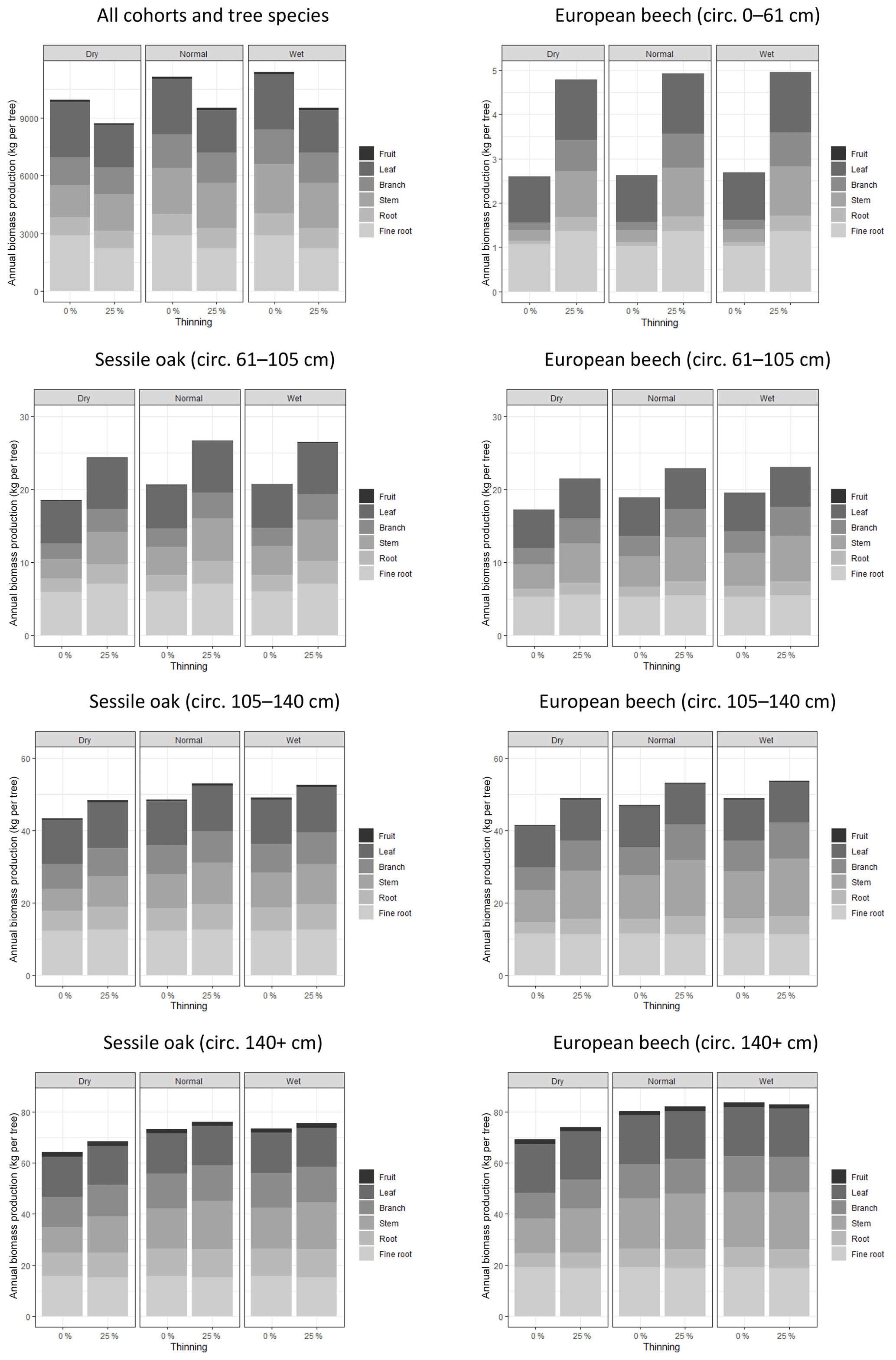
https://www.geosci-model-dev.net/13/905/2020/gmd-13-905-2020-f05

Figure 5Effects of climate conditions and thinning on biomass production and its allocation to tree compartment in the mixed stand in Baileux. The data used to make these graphs were obtained by simulations using the following options: photosynthesis model of CASTANEA, npp to gpp ratio and distance-independent crown extension.

Download

The biomass production at the stand level was 11 % higher for the normal year than for the dry year (Fig. 5). This effect was observed for all of the cohorts even if it was less marked on the smallest trees (+2 % for the 0–61 cm beech cohort) than on the biggest ones (+13 % for oak and beech trees with a girth larger than 140 cm). Whatever the scale considered (tree or stand), there was nearly no difference in biomass production between the normal and wet year. The climate condition effects were marked only on the structural compartment (+25 %).

When the CO₂ concentration of the atmosphere was fixed, no effect of the climate scenario was detected on stand BAI, but a slight impact was observed on sessile oak BAI, which was higher for the RCP2.6 than for the historical scenario (Fig. 6). For the simulations with a variable atmospheric CO₂ concentration, the differences in total, sessile oak and European beech BAIs were much more pronounced among climate scenarios. For the whole stand as well as for oak and beech separately, BAIs increased the following order (1) historical, (2) RCP2.6, (3) RCP4.5 and (4) RCP8.5, with the stand BAI in each of these RCP scenarios being between 17 % and 72 % higher than that of the historical scenario. All of the scenarios had BAIs that were significantly different from each other, except RCP2.6 and RCP4.5 for the whole stand and the two tree species and historical and RCP2.6 for the European beech (Fig. 6).

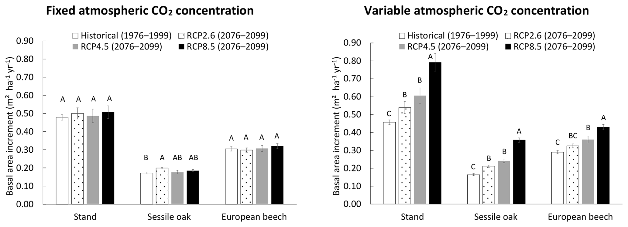
https://www.geosci-model-dev.net/13/905/2020/gmd-13-905-2020-f06

Figure 6Basal area increment (BAI) of the mixed stand in Baileux (and of its two main tree species) simulated with climate scenarios produced with the general circulation model CNRM-CM5, downscaled with ALARO-0 and corrected empirically for remaining biases. The simulations were performed by using the CASTANEA method to calculate photosynthesis, the npp to gpp ratio approach and a distance-independent description of crown extension. The CO₂ concentration of the atmosphere was either kept constant (left) or increased with time according to the climate scenario considered (right). Two time periods were considered. The 1976–1999 period was used as a reference for running the model with the historical climate scenario, while the simulations with future climate scenarios were carried out for the 2076–2099 period. The climate scenarios were based on the representative concentration pathways for atmospheric greenhouse gases that are described in the fifth assessment report of IPPC. For a given tree species and CO₂ concentration modality, the scenarios with common letters have BAIs not significantly different from each other (α=0.05).

Download

4 Discussion

Few tree-level, process-based and spatially explicit models have been developed, and these often contain only some of the modules necessary to estimate resource availability (solar radiation, water and nutrients). While descriptions of these models are generally available in the literature, doing an evaluation by making a comparison with tree growth measurements is not always accessible, or such an evaluation has been carried out based on stand-level variables. We have therefore very little information to compare the performances of HETEROFOR at the tree level with those of similar models. Simioni et al. (2016) faced the same problem with the NOTG 3-D model.

HETEROFOR first estimates the key phenological dates, the radiation interception by trees and the hourly water balance (de Wergifosse et al., 2019). Then, based on the absorbed PAR radiation, individual gpp is calculated with a PUE approach or with the photosynthesis routine of CASTANEA (Dufrêne et al., 2005). Whatever the option retained for calculating tree respiration and crown extension, the photosynthesis routine of CASTANEA and the PUE efficiency approach performed similarly (Table 3). It is quite encouraging that the process-based approach for estimating photosynthesis provided predictions of the same quality as the empirical approach fitted with tree growth data taken on the study site. If no extrapolation to future climate is required, the PUE approach remains however still valuable, especially when hourly meteorological data are lacking. For the three stands in Baileux, we related the npp reconstructed from successive tree inventories with the gpp predicted based on the CASTANEA approach (Fig. 2). The good linear relationships (Pearson's correlation > 0.89) obtained for both oak and beech make us confident in the adaptation of the photosynthesis routine of CASTANEA to the tree level. Furthermore, since the parameters of the photosynthesis routine were taken directly from CASTANEA and not calibrated specifically for HETEROFOR, one can expect that the agreement between the predicted gpp and the reconstructed npp could still be improved.

When comparing the two options available in HETEROFOR for converting gpp into npp, model performances were systematically better with the npp to gpp ratio approach than with the temperature-dependent routine for the maintenance respiration calculation (Table 3). This can be partly explained because the error in the maintenance respiration calculation results from various sources. At the tree compartment level, uncertainties in the estimation of biomass, sapwood proportion, nitrogen concentration and temperature are multiplied (Eq. 11). Then, the errors made on all of the tree compartments are summed up. Among these uncertainty sources, the inaccuracy in the estimation of the sapwood proportion could explain why the maintenance respiration routine provided better results for the sessile oak than for European beech (Table 3). Since the sapwood of sessile oak can easily be distinguish from the heartwood based on the colour change, we had a lot of sapwood measurements available to fit a relationship. For the European beech, this was not the case; instead, we used a sapwood relationship obtained based on sap flow measurements (Jonard et al., 2011). This relationship could certainly be improved by direct measurements of sapwood made after staining the wood to highlight the living parenchyma. Another way to improve these relationships is to consider the social status of the trees since dominant trees have a higher sapwood depth than the suppressed ones (Rodríguez-Calcerrada et al., 2015). We tried to account for this by estimating the sapwood area based on the tree growth rate, but it did not significantly increase the quality of the predictions. The poor performances obtained with the maintenance respiration option also indicate that the processes at play are still poorly understood and that further research is needed on this topic.

The process-based approach for estimating maintenance respiration explicitly accounts for the temperature effect through a Q₁₀ function. With the npp to gpp ratio approach, temperature is considered more indirectly by assuming that it affects respiration and photosynthesis in the same proportion, which is valid only in a given range of temperature (< 20 ^∘C) and for non-stressing conditions. Indeed, the optimum temperature for photosynthesis is between 20 and 30 ^∘C, while the optimum temperature for respiration is just below the temperature of enzyme inactivation (> 45 ^∘C). Therefore, between 30 and 45 ^∘C, photosynthetic rates decrease, but the respiration rate could continue to increase (Yamori et al., 2013). This reasoning however does not consider that the base rate of respiration acclimate to new mean temperature conditions and that this acclimation process tends to maintain the npp to gpp ratio more stably (Collalti and Prentice, 2019). In addition, while water stress reduces both photosynthesis and respiration, its effect on the two processes is not necessarily equivalent (Rodríguez-Calcerrada et al., 2014). The main argument in favour of the npp to gpp ratio approach is the tight coupling between respiration and photosynthesis since the substrate for respiration originates from photosynthesis. The npp to gpp ratio is unfortunately neither universal nor constant. It may vary with tree development stage, climate, soil fertility and competition conditions (Collalti and Prentice, 2019). The alternative option based on maintenance respiration calculation is theoretically more appropriate to simulate the impact of climate change, but this is at the expense of less accurate predictions at the tree level. The ideal is to compare the two options to evaluate the prediction uncertainty associated with the modelling of respiration. In the future, the two approaches could be improved. Applying the reconstruction procedure of HETEROFOR on a large diversity of sites would allow us to estimate the npp to gpp ratio in many different situations, to create a function predicting the npp to gpp ratio based on its main drivers and to subsequently use it in the model. In parallel, the respiration calculation could be refined by accounting for thermal acclimation, such as is done in 3D-CMCC (Collalti et al., 2018).

The differences in prediction quality between the two methods of crown extension modelling (distance-dependent approach vs. distance-independent approach) were quite small, probably because the length of the simulation was not sufficient to drastically affect the crown dimensions, which had been initialized based on measurements. Describing mechanisms that govern crown development in interaction with neighbours (mechanical abrasion and crown interpenetration) is however crucial to capturing the nonadditive effect of species mixtures (Pretzsch, 2014). By accounting for crown plasticity, our distance-dependent approach could help us to better understand how uneven-aged and mixed stands optimize light interception by canopy packing and how they increase productivity (Forrester and Albrecht, 2014; Jucker et al., 2015). To better evaluate the relevance of this approach, the predicted crown development should be compared with precise crown measurements that are repeated over several decades and taken in a large diversity of stand structures. When the model will be calibrated for a larger number of tree species, long-term simulations could also be performed to evaluate to what extent the model is able to reconstruct the empirical relationships that describe tree allometry variations in response to intra- and inter-specific competition. Such relationships were established by del Río et al. (2019) using data from the Spanish National Forest Inventory.

Based on the current evaluation, the process-based variant performs similarly to the more empirical one for photosynthesis and crown extension but not for respiration; this is probably because the processes are better known for photosynthesis. For the best combination of options using the CASTANEA photosynthesis (npp to gpp ratio with distance-dependent crown extension), the Pearson's correlation between measurements and predictions of individual basal increment amounted to 0.83 and 0.63 for European beech and sessile oak, respectively. By comparison, Grote and Pretzsch (2002) obtained a correlation of 0.60 for the individual volume of beech trees with the BALANCE model. This lower correlation can partly be explained by the integration of the uncertainty in tree height in the volume estimations.

Individual npp and retranslocated carbon are allocated first to foliage and fine roots and then partitioned between above- and below-ground structural compartments. Based on the derivative and rearrangement of a biomass allometric equation, the increment in aboveground structural biomass is used to estimate the combined increment in dbh and height. This results in a system of one equation with two unknowns (increment in dbh and height). We decided to resolve it by fixing the height growth based on a relationship that takes into account tree size (dbh or height), the height growth potential (height increment if all of the remaining carbon was allocated to height growth) and a light competition index. An intermediate level of sophistication was adopted to describe height growth, between the simple height–dbh allometry and the fine description of tree architecture of functional–structural models. Height–dbh relationships provide a static picture in which age and neighbour effects are confounded and are not suitable to describe individual growth trajectories (Henry and Aarsen, 1999). More sophisticated relationships considering age and dominant height can be used for even-aged stands (Le Moguédec and Dhôte, 2012) but are hardly applicable in uneven-aged stands for which tree age is unknown. On the other hand, the functional–structural models that are based on resource availability at the organ level and use a short time step can only be applied to a limited number of trees given the high computational demand (Letort et al., 2008).

Our individual height growth model was fitted with height data measured 10 years apart (Appendix E). A large uncertainty was however associated to these data. First, height measurements were obtained to the nearest metre given the difficulty to clearly identify the top of the trees in closed canopy forests. Second, as the height increment was obtained based on repeated height measurements, the error for this variable is the sum of those made on the height measurements. Consequently, the uncertainty was more or less of the same order of magnitude as the expected height growth in 10 years. Despite these uncertainties, a substantial part of the variability was explained by the model (72 % for European beech; 43 % for oak). Among the variables tested, the height growth potential had the main effect, which is not surprising since this height growth potential contains the information on height increment. We were also able to depict the effect of light competition. For a same-height growth potential, trees undergoing stronger light competition seem to invest more carbon for height growth than for dbh increment (Fig. E1 in Appendix E), which is corroborated by results of other studies (e.g. Lines et al., 2012). This strategy aims at minimizing overtopping by neighbours and maximizing light interception (Jucker et al., 2015). Trouvé et al. (2015) found similar results and showed the positive effect of stand density on height growth in the allocation between height and diameter increment in even-aged stands of sessile oak trees. The decrease in the red : far red ratio of incident light promotes apical dominance and internode elongation through the phytochrome system (shade avoidance reaction; Henry and Aarsen, 1999). By considering the light availability effect on height growth at the tree level, HETEROFOR adapts tree allometry to intra- and inter-specific competition, which is crucial to accounting for mixing effects in structurally complex stands (del Río et al., 2019).

A first simulation experiment was achieved to assess how tree biomass production and its allocation to tree compartments respond to climate conditions and thinning. The results of these simulations are in line with the basic principles of silviculture; thinning favoured individual tree growth (especially that of the smaller trees) by redistributing stand biomass production on a smaller number of trees. At the stand level, thinning slightly reduced biomass production since its intensity was substantial and the simulation lasted only 1 year, which was not sufficient to allow the remaining trees to fill the gaps by extending their crown. Drought conditions reduced the biomass increment of structural components, and this effect was more pronounced on big trees than on small trees. Indeed, when soil water availability decreases, smaller trees maintain a higher stomatal conductivity because of their lower position in the stand canopy. Functional compartments were less influenced by climate because carbon is allocated to them in priority in the model. We could improve the allocation routine by making the fine root to foliage ratio and the root-to-shoot ratio dependent on the mean soil water availability (Thurm et al., 2017).

We were also quite satisfied to observe that the model was able to reproduce the size–growth relationship. This approach describes the growth partitioning among trees in a stand, which is useful to estimate the mode of competition. For the three studied stands and the two tree species, the competition was partially size asymmetric, with a resource partitioning in favour of the larger trees (Carl et al., 2018). Within the studied stands, the European beech trees can be classified in two groups: a group of small suppressed trees whose radial growth was close to 0 and which were just surviving and the rest of the trees (beyond a girth threshold) whose radial growth linearly increased with girth. Regarding sessile oaks, nearly all of the trees were in the second group, which can be related to the fact that sessile oak is a less shade-tolerant species than European beech. In the this mixed stand, the nearly perfect match between the predicted and observed relationships indicates that the model was able to reproduce growth partitioning among trees of different tree species and size. These very good results can be ascribed to the fact that the extinction coefficient and the respiration parameters were calibrated with data from this stand. In the beech-dominated stand, the model slightly underestimated the radial growth of the small oak trees and overestimated that of the big beech trees. In this case, the model seems to allocate too many resources to the big beech trees which shade the small oak trees. This could be improved by a model calibration partly specific to this stand (for the npp to gpp ratio) or by a calibration with data covering a much larger range of stand structures.

To illustrate one possible application of HETEROFOR, a second simulation experiment was completed and allowed us to compare the radial growth predicted for 2076–2099 according to three IPCC scenarios with that of the one simulated for an historical period (1976–1999). When the atmospheric CO₂ concentration was kept constant (380 ppm), differences among scenarios remained nonsignificant, except for sessile oak displaying a slightly higher basal area increment for the RCP2.6 scenario than for the historical scenario (Fig. 6). Analysing the model outputs in depth, we found that this lack of effects resulted from a balance between negative and positive impacts of climate change. While the increase in air temperature (+0.9 and 3.7 ^∘C for RCP2.6 and RCP8.5) and in the vegetation period length (+8 and 37 days for RCP2.6 and RCP8.5) favoured photosynthesis, the more frequent and intense water stress negatively affected it (de Wergifosse et al., 2020). The positive and negative effects of climate change were of the same magnitude for both tree species and offset each other. For the simulations with a variable atmospheric CO₂ concentration, the differences among scenarios were much larger, highlighting a strong CO₂ fertilization effect for both sessile oak and European beech (Fig. 6). These results are in agreement with Reyer et al. (2014), which used the 4C model to predict productivity change in Europe according to a large range of climate change projections. They found npp increases in most European regions (except a few cases in Mediterranean mountains) when considering persistent CO₂ effects by using a variable atmospheric CO₂ concentration. Assuming an acclimation of photosynthesis to CO₂ (by maintaining constant atmospheric CO₂), they predicted increases in northern Europe, decreases in southern Europe and ambivalent responses elsewhere in Europe. Similar response patterns were also obtained by Morales et al. (2007). Rötzer et al. (2013) used the BALANCE model to compare the impact of future and current climate conditions on the productivity of beeches in Germany and showed a 30 % decrease in npp without considering the rise in atmospheric CO₂ concentration. After evaluating CASTANEA against eddy covariance and tree growth data in a few highly instrumented sites, Davi et al. (2006) simulated the trend in gpp and net ecosystem productivity (NEP) in these sites from 1960 to 2100. For sessile oak and European beech, they obtained a 53 % and 67 % increase in gpp and NEP, respectively.

Given the magnitude of the CO₂ fertilization effect (leading to a 72 % increase in basal area increment in 100 years for RCP8.5), we conducted retrospective simulations to check that HETEROFOR reproduces well the increase in productivity observed by Bontemps et al. (2011) for beech forests in the north-east of France (data not shown). Based on historical atmospheric CO₂ concentrations, we simulated radial growth during two periods (1879–1910 vs. 1979–2010) using the same climate data (obtained by reanalysis for 1979–2010). These simulations showed a productivity increase of 12 % over 100 years. By comparison, Bontemps et al. (2011) reported productivity increases ranging from 10 to 70 % over 100 years, depending on the nitrogen status of the forest. The increase in radial growth simulated with HETEROFOR for the mixed stand in Baileux (Fig. 6) seems therefore plausible but assumes unchanged nutritional status. Increased productivity generates however higher nutrient demand by trees, which is not systematically satisfied by larger soil nutrient supply, especially in the poorest sites. Consequently, the augmentation of forest productivity will most likely be constrained by nutrient availability and give rise to a deterioration of the nutritional status as already observed across Europe (Jonard et al., 2015). To improve our predictions, nutritional constraints must be taken into account. From this perspective, a mineral nutrition and nutrient cycle module was incorporated in HETEROFOR. As it was developed in parallel to the water balance, some adaptations are needed for the coupling of the two modules (e.g. change from an annual to a monthly time step for soil chemistry update). A complete description and evaluation of the nutrient module will be provided in a future study.

5 Conclusion and future prospects

Our ambition was to develop a model that is responsive to both management actions and environmental changes and would be particularly well adapted to mixed and uneven-aged stands. We thought that this model had to be tree-level and spatially explicit and had to consider radiation transfer, water balance and nutrient cycling with a process-based approach. Such models were very scarce in the literature. The only exceptions were BALANCE, iLand and more recently NOTG 3-D. To fill this gap, we elaborated the HETEROFOR model based on concepts quite different from those used for BALANCE, iLand and NOTG 3-D. In this study, a first evaluation of the model performances showed that HETEROFOR was able to reproduce size–growth relationships in three oak and beech stands in the Belgian Ardennes. We also noticed that the npp to gpp ratio option for describing maintenance respiration provides the best results, while the process-based and empirical approaches perform similarly for photosynthesis and crown extension. As this model evaluation was limited to two tree species and one climate, it only provides a first impression of the model potential.

Here, only the core of HETEROFOR was described. The water balance and phenology modules are presented and evaluated in a companion paper (de Wergifosse et al., 2019), while the nutrient module will be described later. For the next steps, we plan to couple HETEROFOR with existing libraries such as the ones for regeneration, genetics and economics. As HETEROFOR was developed within the Capsis platform, it is continually improving thanks to the collaborative dynamics among modellers.

A broader assessment of the model performances will be carried out based on forest monitoring plots distributed all over Europe. Indeed, HETEROFOR was designed to be particularly suitable for the level II plots of ICP Forests. The processes were described at a scale that facilitates the comparison between model predictions and observations. Many data collected in these plots can be used to initialize and run the model or to calibrate and evaluate it. HETEROFOR can also be seen as a tool for integrating forest monitoring data and quantifying non-measured processes. While it is now calibrated for oak and beech forests, HETEROFOR will be parameterized for a large range of tree species in order to use it for testing and reproducing identity and diversity effects.

Given all of the uncertainties related to climate change impacts, it is unrealistic to believe that a model will accurately predict the future dynamics of forest growth. However, models such as HETEROFOR can be very useful to compare scenarios. Among others purposes, HETEROFOR can be used to select the management options that maximize ecosystem resilience or to quantify uncertainty in the response of forest ecosystem to climate change.

Appendix A: Description of the soil heat transfer routine

The temperature of the mineral soil (T; in degrees Celsius) is calculated by soil depth increment (Δz; in metres) using a simplification of the soil heat transfer equation assuming a constant thermal diffusivity (D; in square metres per second) across the soil profile. The thermal diffusivity characterizes the rate of heat transfer within the soil and corresponds to the ratio of the thermal conductivity (K; in watts per metre per kelvin) to the volumetric heat capacity (c_v; in joules per cubic metre per kelvin).

\begin{matrix} (A1) & \frac{\partial T}{\partial t} = \frac{1}{c_{v}} \cdot \frac{\partial}{\partial z} \cdot (K \frac{\partial T}{\partial z}) = > \frac{\partial T}{\partial t} = D \cdot \frac{\partial^{2} T}{\partial z^{2}} \end{matrix}

Eq. (A1) can be rewritten according to Anlauf and Liu (1990) and Baker and Don Scott (1998) as follows:

\begin{matrix} (A2) & T_{z, t + Δ t} = T_{z, t} + D \cdot \frac{Δ t}{Δ z^{2}} \cdot (T_{z + Δ z, t} + T_{z - Δ z, t} - 2 T_{z, t}) . \end{matrix}

The soil depth increment can be chosen by the user, but it has to be smaller than one-third of the thinnest horizon. The soil depth increment can be slightly modified by the model to ensure that the soil depth is a multiple of the soil depth increment. Then, a stability criterion is checked for each hour, and if it is not respected, the temporal step is divided by two.

\begin{matrix} (A3) & K \cdot \frac{Δ T}{Δ z^{2}} < 0.5 \end{matrix}

The thermal diffusivity is calculated for each soil horizon based on the thermal conductivity and the volumetric heat capacity and then averaged by weighing according the horizon thickness. The thermal conductivity is obtained with the empirical model of Kersten (1949) as follows:

\begin{matrix} (A4) & \begin{aligned} K = 0.1442 \cdot (0.9 \cdot \log (ϑ) - 0.2) \times 10^{0.6243 ρ_{b}} \\ (for silt or clay soils) \end{aligned} \\ (A5) & \begin{aligned} K = 0.1442 \cdot (0.7 \cdot \log (ϑ) + 0.4) \times 10^{0.6243 ρ_{b}} \\ (for sandy soils), \end{aligned} \end{matrix}

with ϑ, the gravimetric soil water content (in grams per gram), and ρ_b, the bulk density (in kilograms per cubic metre)

The volumetric heat capacity of soils is approximated through a separation of the soil constituents in solid and liquid phases as follows:

\begin{matrix} (A6) & c_{v} ≃ 836 \cdot ρ_{b} + 4180 \cdot ϑ \cdot ρ_{b} \cdot 1000 \cdot ρ_{w}, \end{matrix}

with ρ_w, the volumetric mass of water (in kilograms per cubic metre).

To initialize the procedure, the top and bottom temperature during the whole simulation and the initial temperature at each soil depth must be known. The soil temperature at the top of the mineral soil (just under the forest floor) is given by Eq. (A7) adapted from van Wijk and de Vries (1963) and Cichota et al. (2004). The bottom temperature is fixed and corresponds to the mean annual air temperature. This assumption can be made as the soil depth largely exceeds 1 m. The initial temperature is found through a simple interpolation of the temperatures between the soil interface and the bottom.

\begin{matrix} (A7) & \begin{aligned} T_{t} = & {\overline{T}}_{y} + \frac{({\overline{T}}_{d - 1} - {\overline{T}}_{y})}{A_{air}} \cdot A_{soil} + \frac{a_{air}}{2} \cdot {red}_{d} \\ \cdot \sin (ω (t - t_{T_{\max}}) + \frac{π}{2} - ω \frac{Δ z}{Damping}), \end{aligned} \end{matrix}

with ${\overline{T}}_{y}$ , mean annual air temperature (in degrees Celsius), ${\overline{T}}_{d - 1},$ mean air temperature of the previous day (in degrees Celsius), A_air, annual air temperature amplitude corresponding to the difference between the maximum and the minimum mean daily temperature over the year (in degrees Celsius), A_soil, a parameter corresponding to the mean annual soil temperature amplitude (in degrees Celsius), a_air, daily air temperature amplitude (T_max−T_min) calculated over the 24 h period centred on the considered time (^∘C), red_d, parameter reducing the daily air temperature amplitude to the daily soil temperature amplitude (fixed to 0.13), ω, radial frequency (per hour) is $\frac{2 π}{24}$ , $t_{T_{\max}}$ , hour of the day at which air temperature is maximal (as the sinusoidal shape of the diurnal soil temperature cycle is not perfectly symmetric, $t_{T_{\max}}$ is adapted so that the period between maximum and minimum soil temperature is exactly 12 h), Δz, thickness of organic horizons (in metres), and Damping, a parameter accounting for the phase shift between the diurnal cycle of the air and soil temperature (fixed to 0.0853 after calibration).

The temperature of the organic horizons was obtained as the mean between air temperature and the temperature at the interface between organic horizons and mineral soil.

Appendix B: Development of Eq. (29)

Equation (29) can be developed in order to isolate Δh as follows:

\begin{matrix} (B1) & \begin{aligned} Δ ({dbh}^{2} \cdot h) = & (dbh + Δ dbh)^{2} \cdot (h + Δ h) - {dbh}^{2} \cdot h \\ Δ ({dbh}^{2} \cdot h) = & ({dbh}^{2} + 2 \cdot dbh \cdot Δ dbh + (Δ dbh)^{2}) \\ \cdot (h + Δ h) - {dbh}^{2} \cdot h \end{aligned} \\ (B2) & \begin{aligned} Δ ({dbh}^{2} \cdot h) = & {dbh}^{2} \cdot h + 2 \cdot dbh \cdot Δ dbh \cdot h + {(Δ dbh)}^{2} \\ \cdot h + {dbh}^{2} \cdot Δ h + 2 \cdot dbh \cdot Δ dbh \\ \cdot Δ h + {(Δ dbh)}^{2} \cdot Δ h - {dbh}^{2} \\ \cdot h Δ ({dbh}^{2} \cdot h) \\ = & Δ {dbh}^{2} \cdot (h + Δ h) + {(Δ dbh)}^{2} \\ \cdot (h + Δ h) + {dbh}^{2} \cdot Δ h \end{aligned} \\ (B3) & \begin{aligned} Δ ({dbh}^{2} \cdot h) = & Δ h \cdot (Δ {dbh}^{2} + {(Δ dbh)}^{2} + {dbh}^{2}) + h \\ \cdot (Δ {dbh}^{2} + {(Δ dbh)}^{2}) . \end{aligned} \end{matrix}

Considering $(Δ dbh)^{2} ≪ Δ {dbh}^{2} ≪ dbh$ , an approximation can be done as follows:

\begin{array}{l} (B4) & Δ ({dbh}^{2} \cdot h) ≅ Δ h \cdot {dbh}^{2} + h \cdot Δ {dbh}^{2} \\ (B5) & Δ h \cdot {dbh}^{2} ≅ Δ ({dbh}^{2} \cdot h) - h \cdot Δ {dbh}^{2} \\ (B6) & Δ h ≅ \frac{Δ ({dbh}^{2} \cdot h)}{{dbh}^{2}} - \frac{h \cdot Δ {dbh}^{2}}{{dbh}^{2}} . \end{array}

Appendix C: Delevoy height estimation

The Delevoy height is the height at which stem diameter is half the diameter at breast height and is calculated from taper (in centimetres per metre) as follows:

\begin{matrix} (C1) & h_{del} = 1.3 + \frac{dbh - \frac{dbh}{2}}{taper}, \end{matrix}

where the taper is obtained based on the girth at 10 % of the tree height (G10%) and the relative girth at 60 % of the tree height (RG60%) for which empirical equations are provided by Dagnelie et al. (1999) for several temperate tree species.

\begin{matrix} (C2) & taper = \frac{(1 - CR60%) \cdot C10%}{0.5 \cdot h \cdot π}, \end{matrix}

with

\begin{matrix} (C3) & \begin{aligned} C10% = & a + b \cdot π \cdot dbh + c \cdot {(π \cdot dbh)}^{2} + d \cdot (π \cdot dbh)^{3} \\ + e \cdot h + f \cdot (π \cdot dbh)^{2} \cdot h \end{aligned} \\ (C4) & CR60% = a + \frac{b}{C10%} + \frac{c}{{C10%}^{2}} . \end{matrix}

Table C1Parameters of Eqs. (C3) and (C4) for sessile oak and European beech according to Dagnelie et al. (1999).

Download Print Version | Download XLSX

Appendix D: Estimation of the height of largest crown extension (hlce) at equilibrium

https://www.geosci-model-dev.net/13/905/2020/gmd-13-905-2020-f07

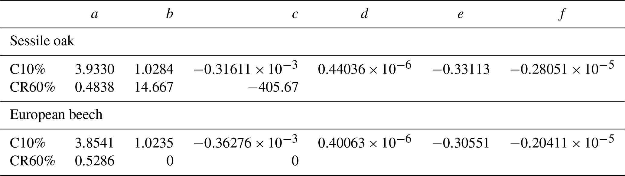
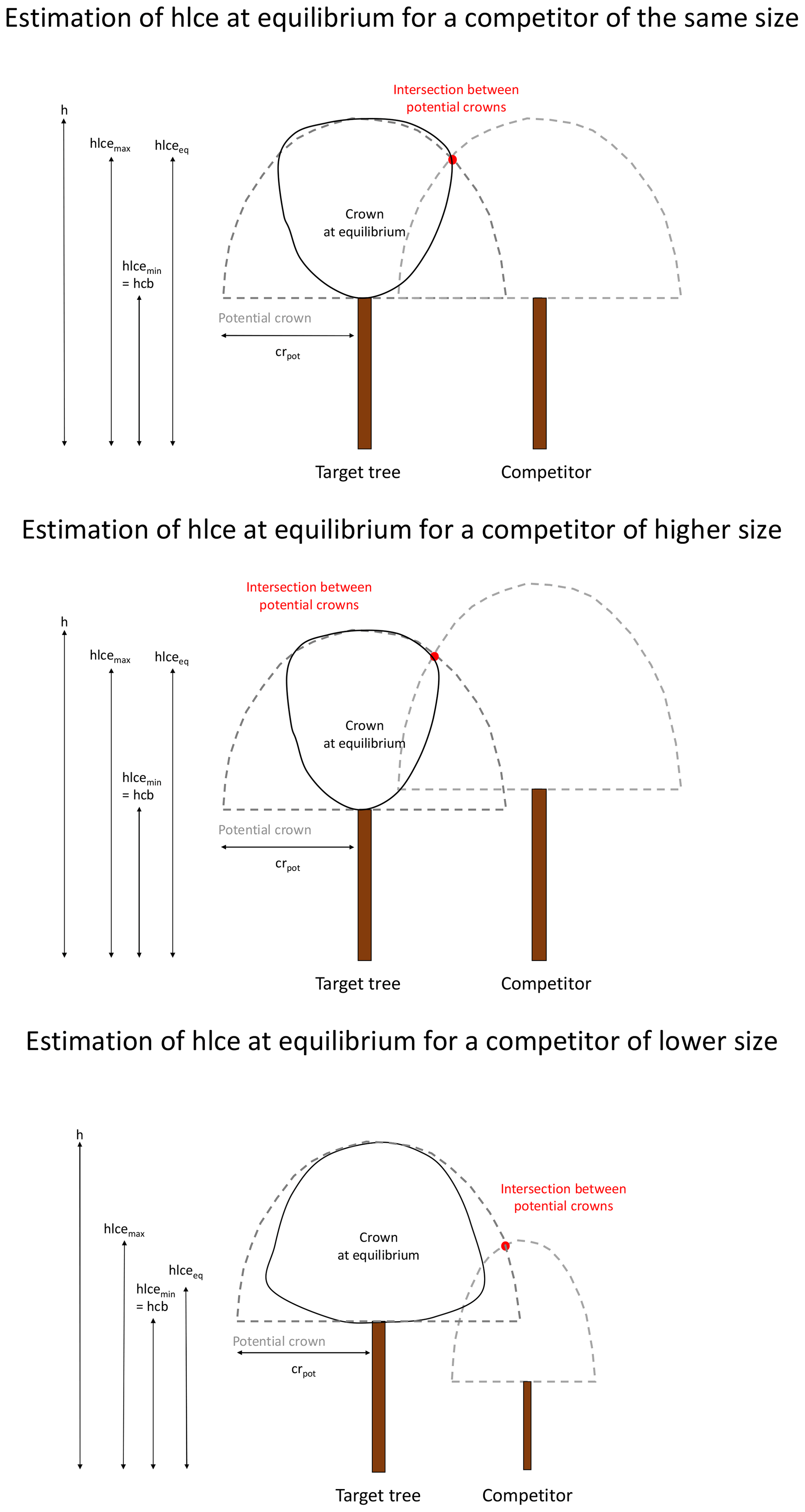
Figure D1Illustration of the routine used to determine the height of largest crown extension at equilibrium (hlce_eq) of a target tree in three contrasting situations of competition. A first step consists in determining the intersection between the potential crown of the target tree and the competitor. Then, the hlce_eq is fixed between the maximum hlce (corresponding to the intersection between potential crowns) and the minimum hlce (which is the height to crown base) based on the relative height of the competitor.

Download

Appendix E: Height growth modelling results

The main factor explaining the height increment was the so-called height growth potential (Δh_pot), with a quadratic effect for beech and a cubic effect for oak (Table E1 and Fig. E1). For both tree species, the light competition index (LCI) had a negative effect on the height increment, meaning that, for a same-height growth potential, trees under stronger competition for light had a higher height growth than trees within better light conditions. For the European beech, the variable selection procedure selected height (which had a negative effect) to account for tree size, while dbh was retained for sessile oak and had a positive effect. Even if the root-mean-square error was slightly higher for European beech (0.094) than for sessile oak (0.083), the height growth model explained a much larger proportion of the variability in European beeches (72 %) than in sessile oaks (43 %). This is partly because the height growth range was higher for European beeches.

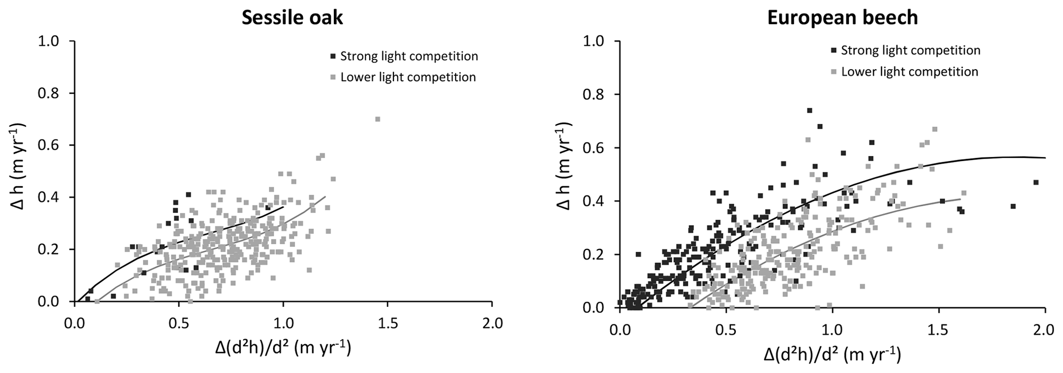
https://www.geosci-model-dev.net/13/905/2020/gmd-13-905-2020-f08

Figure E1Effect of the height growth potential on oak and beech height growth for two levels of light competition (strong light competition = light competition index ≤ 0.15, lower light competition = light competition index > 0.15). The solid lines represent the model predictions obtained using Eq. (31) with parameter values of Table E1 and with mean values for dbh, height or the light competition index.

Download

Table E1Parameters, R² and RMSE of the height growth model (Eq. 31) for European beech and sessile oak.

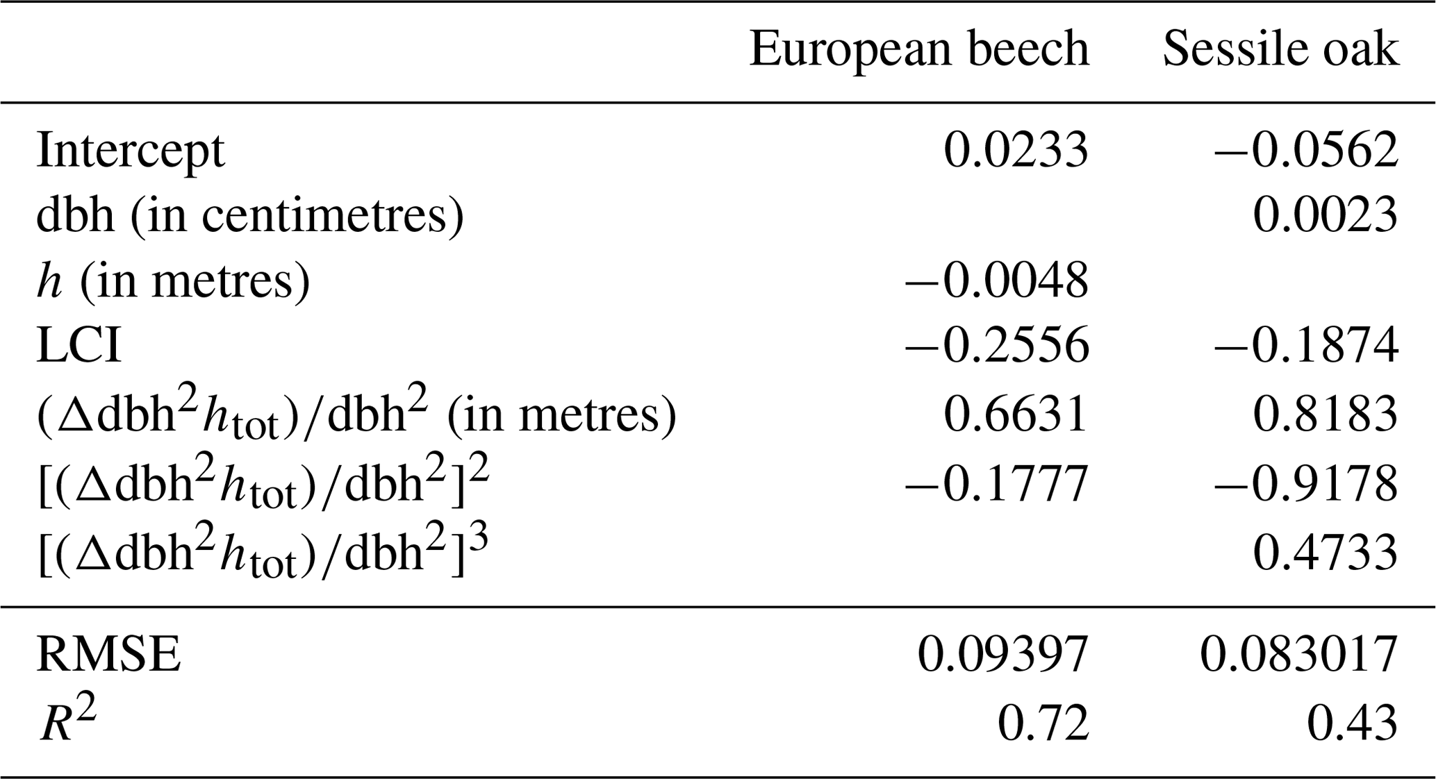
Download Print Version | Download XLSX

Code availability

The source codes of Capsis and HETEROFOR are accessible to all of the members of the Capsis co-development community. Those who want to join this community are welcome but must contact François de Coligny (coligny@cirad.fr) and sign the Capsis charter (http://capsis.cirad.fr/capsis/charter, last access: 29 February 2020). This charter grants access on all the models to the modellers of the Capsis community. The modellers may distribute the Capsis platform with their own model but not with the models of the others without their agreement. Capsis4 is a free software (LGPL licence) which includes the kernel, the generic pilots, the extensions and the libraries. For HETEROFOR, we also choose an LGPL license and decided to freely distribute it through an installer containing the Capsis4 kernel and the latest version (or any previous one) of HETEROFOR upon request from Mathieu Jonard (mathieu.jonard@uclouvain.be). The version 1.0 used for this paper is available at http://amap-dev.cirad.fr/projects/capsis/files (last access: 29 February 2020, Jonard et al., 2020). The end users can install Capsis from an installer containing only the HETEROFOR model, while the modellers who signed the Capsis charter can access to the complete version of Capsis with all of the models. Depending on your status (end user vs modeller or developer), the instructions to install Capsis are given on the Capsis website (http://capsis.cirad.fr/capsis/documentation, last access: 29 February 2020).

The source code for the modules published in Geoscientific Model Development can be downloaded from https://doi.org/10.5281/zenodo.3591348 (Jonard et al., 2019).

Data availability

The data used in this paper are available through the input files for HETEROFOR which are embedded in the installer (see Code availability).

Supplement

The supplement related to this article is available online at: https://doi.org/10.5194/gmd-13-905-2020-supplement.

Author contributions

MJ, FA, FdC, LdW, NB and HD developed the model code. FA carried out the calibration. MJ, FA and LdW performed the simulations and analysed the model outputs. MJ prepared the paper with contributions from all coauthors.

Competing interests

The authors declare that they have no conflict of interest.

Acknowledgements

We are grateful to the RMI (Royal Meteorological Institute of Belgium) for providing us climate projection data for the Baileux site. We also would like to thank the four anonymous reviewers for their constructive comments which helped us to significantly improve the quality of the paper.

Financial support

This research has been supported by the Service Public de Wallonie (SPW/DGO 3/DNF) (Accord-Cadre de Recherche et Vulgarisation Forestières 2014–2019), the Fonds de la Recherche Scientifique – FNRS (PDR-WISD grant no. 09; the SustainFor project) and the Fonds de la Recherche Scientifique – FNRS, Fonds pour la Formation à la Recherche dans l'Industrie et dans l'Agriculture (grant no. 1.E005.18).

Review statement

This paper was edited by Min-Hui Lo and reviewed by Rüdiger Grote and three anonymous referees.

References

Aber, J., Neilson, R. P., McNulty, S., Lenihan, J. M., Bachelet, D., and Drapek, R. J.: Forest processes and global environmental change: predicting the effects of individual and multiple stressors, Bioscience, 51, 735–751, 2001.

André, F., Jonard, M., and Ponette, Q.: Precipitation water storage capacity in a temperate mixed oak–beech canopy, Hydrol. Process., 22, 4130–4141, 2008a.

André, F., Jonard, M., and Ponette, Q.: Influence of species and rain event characteristics on stemflow volume in a temperate mixed oak–beech stand, Hydrol. Process., 22, 4455–4466, 2008b.

André, F., Jonard, M., and Ponette, Q.: Biomass and nutrient content of sessile oak (Quercus petraea (Matt.) Liebl.) and beech (Fagus sylvatica L.) stem and branches in a mixed stand in southern Belgium, Sci. Total Environ., 408, 2285–2294, 2010.

André, F., Jonard, M., Jonard, F., and Ponette, Q.: Spatial and temporal patterns of throughfall volume in a deciduous mixed-species stand, J. Hydrol., 400, 244–255, 2011.

Anlauf, R. and Liu, Y. P.: Simulation of simple one-dimensional transport processes, in: Models for Processes in the Soil: Programs and Exercises, edited by: Richter, J., Catena Verlag, Cremlingen-Desdedt, Germany, 1990.

Baker, D. L. and Don Scott, H.: A limited tutorial on using finite differences in soil physics problems, available at: http://www.aquarien.com/findif/Findifa4.html (last access: 29 February 2020), 1998.

Ball, J. T., Woodrow, I. E., and Berry, J. A.: A model predicting stomatal conductance and its contribution to the control of photosynthetis under different environmental conditions, in: Progress in Photosynthesis Research, edited by: Biggins, J., vol. 4, 221–224, 1987.

Berger, U., Piou, C., Schiffers, K., and Grimm, V.: Competition among plants: concepts, individual-based modelling approaches, and a proposal for a future research strategy, Perspect. Plant Ecol., 9, 121–135, 2008.

Boisvenue, C. and Running, S. W.: Impacts of climate change on natural forest productivity–evidence since the middle of the 20th century, Glob. Change Biol., 12, 862–882, 2006.

Bontemps, J. D., Hervé, J. C., Leban, J. M., and Dhôte, J. F.: Nitrogen footprint in a long-term observation of forest growth over the twentieth century., Trees, 25, 237–251, 2011.

Bosc, A.: EMILION, a tree functional-structural model: presentation and first application to the analysis of branch carbon balance, Ann. Forest Sci., 57, 555–569, 2000.

Bravo, F., Fabrika, M., Ammer, C., Barreiro, S., Bielak, K., Coll, L., Fonseca, T., Kangur, A., Löf, M., Merganicova, K., Pach, M., Pretzsch, H., Stojanovic, D., Schuler, L., Peric, S., Rötzer, T., del Rio, M., Dodan, M., and Bravo-Oviedo, A.: Modelling approaches for mixed forests dynamics prognosis, Research gaps and opportunities, Forest Syst., 28, eR002, doi:10.5424/fs/2019281-14342, 2019.

Campioli, M., Vincke, C., Jonard, M., Kint, V., Demarée, G., and Ponette, Q.: Current status and predicted impact of climate change on forest production and biogeochemistry in the temperate oceanic European zone: review and prospects for Belgium as a case study, J. Forest Res., 17, 1–18, 2012.

Cantarello, E., Newton, A. C., Martin, P. A., Evans, P. M., Gosal, A., and Lucash, M. S.: Quantifying resilience of multiple ecosystem services and biodiversity in a temperate forest landscape, Ecol. Evol., 7, 9661–9675, 2017.

Carl, C., Biber, P., Veste, M., Landgraf, D., and Pretzsch, H.: Key drivers of competition and growth partitioning among Robinia pseudoacacia L. trees, Forest Ecol. Manage., 430, 86–93, 2018.

Charlton, S. R. and Parkhurst, D. L.: Modules based on the geochemical model PHREEQC for use in scripting and programming languages, Comput. Geosci., 37, 1653–1663, 2011.

Cichota, R., Elias, E. A., and van Lier, Q. D. J.: Testing a finite-difference model for soil heat transfer by comparing numerical and analytical solutions, Environ. Model. Softw., 19, 495–506, 2004.

Collalti, A., Trotta, C., Keenan, T. F., Ibrom, A., Bond-Lamberty, B., Grote, R., Vicca, S., Reyer, C. P. O., Migliavacca, M., Veroustraete, F., Anav, A., Campioli, M., Scoccimarro, E., Šigut, L., Grieco, E., Cescatti, A., and Matteucci G.: Thinning can reduce losses in carbon use efficiency and carbon stocks in managed forests under warmer climate, J. Adv. Model. Earth Sy., 10, 2427–2452, 2018.

Collalti, A. and Prentice, I. C.: Is NPP proportional to GPP? Waring's hypothesis 20 years on, Tree Physiol. 39, 1473–1483, 2019.

Collins, M., Knutti, R., Arblaster, J., Dufresne, J. L., Fichefet, T., Friedlingstein, P., Gao, X., Gutowski, W. J., Johns, T., Krinner, G., Shongwe, M., Tebaldi, C., Weaver, A. J., and Wehner, M.: Long-term Climate Change: Projections, Commitments and Irreversibility, in: Climate Change 2013: The Physical Science Basis, Contribution of Working Group I to the Fifth Assessment Report of the Intergovernmental Panel on Climate Change, edited by: Stocker, T. F., Qin, D., Plattner, G. K., Tignor, M., Allen, S. K., Boschung, J., Nauels, A., Xia, Y., Bex, V., Midgley, P. M., Cambridge University Press, Cambridge, UK, New York, NY, USA, 2013.

Courbaud, B., de Coligny, F., and Cordonnier, T.: Simulating radiation distribution in a heterogeneous Norway spruce forest on a slope, Agr. Forest Meteorol., 116, 1–18, 2003.

Dagnelie, P., Palm, R., Rondeux, J., and Thill, A.: Tables de cubage des arbres et des peuplements forestiers, Les Presses Agronomiques de Gembloux, Gembloux, Belgique, 1999.

Damesin, C., Ceschia, E., Le Goff, N., Ottorini, J. M., and Dufrêne, E.: Stem and branch respiration of beech: from tree measurements to estimations at the stand level, New Phytol., 153, 159–172, 2002.

Davi, H., Dufrêne, E., Francois, C., Le Maire, G., Loustau, D., Bosc, A., Rambal, S., Granier, A., and Moors, E.: Sensitivity of water and carbon fluxes to climate changes from 1960 to 2100 in European forest ecosystems, Agr. Forest Meteorol., 141, 35–56, 2006.

Davi, H., Cailleret, M., Restoux, G., Amm, A., Pichot, C., and Fady, B.: Disentangling the factors driving tree reproduction, Ecosphere, 7, e01389, https://doi.org/10.1002/ecs2.1389, 2016.

del Río, M., Bravo-Oviedo, A., Ruiz-Peinado, R., and Condés, S.: Tree allometry variation in response to intra- and inter-specific competitions, Trees, 33, 121–138, 2019.

de Wergifosse, L., André, F., Beudez, N., de Coligny, F., Goosse, H., Jonard, F., Ponette, Q., Titeux, H., Vincke, C., and Jonard, M.: HETEROFOR 1.0: a spatially explicit model for exploring the response of structurally complex forests to uncertain future conditions. II. Phenology and water cycle, Geosci. Model Dev. Discuss., https://doi.org/10.5194/gmd-2019-201, in review, 2019.

de Wergifosse, L., André, F., Goosse, H., Caluwaerts, S., De Cruz, L., De Troch, R., and Van Schaeybroeck, B.: CO₂ fertilization, water deficit and vegetation period drive the response of mixed broadleaved forests to a changing climate in Wallonia, Ann. Forest Sci., in review, 2020.

Dufour-Kowalski, S., Courbaud, B., Dreyfus, P., Meredieu, C., and de Coligny, F.: Capsis: an open software framework and community for forest growth modelling, Ann. Forest Sci., 69, 221–233, 2012.

Dufrêne, E., Davi, H., François, C., Le Maire, G., Le Dantec, V., and Granier, A.: Modelling carbon and water cycles in a beech forest: Part I: Model description and uncertainty analysis on modelled NEE, Ecol. Model., 185, 407–436, 2005.

Duursma, R. A. and Medlyn, B. E.: MAESPA: a model to study interactions between water limitation, environmental drivers and vegetation function at tree and stand levels, with an example application to [CO₂] × drought interactions, Geosci. Model Dev., 5, 919–940, https://doi.org/10.5194/gmd-5-919-2012, 2012.

Ennos, R., Cottrell, J., Hall, J., and O'Brien, D.: Is the introduction of novel exotic forest tree species a rational response to rapid environmental change? – A British perspective, Forest Ecol. Manag., 432, 718–728, 2019.

Epron, D., Le Dantec, V., Dufrêne, E., and Granier, A.: Seasonal dynamics of soil carbon efflux and simulated rhizosphere respiration in a beech forest, Tree Physiol., 21, 145–152, 2001.

Farquhar, G. D., von Caemmerer, S., and Berry, J. A.: A biochemical model of photosynthetic CO₂ assimilation in leaves of C3 species, Planta, 149, 78–80, 1980.

Fernandez-Martinez, M., Vicca, S., Janssens, I. A., Sardans, J., Luyssaert, S., Campioli, M., Chapin III, F. S., Ciais, P., Malhi, Y., Obersteiner, M., Papale, D., Piao, S. L., Reichstein, M., Rodà, F., and Peñuelas, J.: Nutrient availability as the key regulator of global forest carbon balance. Nat. Clim. Change, 4, 471–476, 2014.

Forrester, D. I. and Albrecht, A. T.: Light absorption and light-use efficiency in mixtures of Abies alba and Picea abies along a productivity gradient, Forest Ecol. Manag., 328, 94–102, 2014.

Genet, H., Bréda, N., and Dufrêne, E.: Age-related variation in carbon allocation at tree and stand scales in beech (Fagus sylvatica L.) and sessile oak (Quercus petraea (Matt.) Liebl.) using a chronosequence approach, Tree Physiol., 30, 177–192, 2010.

Genet, A., Wernsdörfer, H., Jonard, M., Pretzsch, H., Rauch, M., Ponette, Q., Nys, C., Legout, A., Ranger, J., Vallet P., and Saint-André, L.: Ontogeny partly explains the apparent heterogeneity of published biomass equations for Fagus sylvatica in central Europe, Forest Ecol. Manag., 261, 1188–1202, 2011.

Giot, O., Termonia, P., Degrauwe, D., De Troch, R., Caluwaerts, S., Smet, G., Berckmans, J., Deckmyn, A., De Cruz, L., De Meutter, P., Duerinckx, A., Gerard, L., Hamdi, R., Van den Bergh, J., Van Ginderachter, M., and Van Schaeybroeck, B.: Validation of the ALARO-0 model within the EURO-CORDEX framework, Geosci. Model Dev., 9, 1143–1152, https://doi.org/10.5194/gmd-9-1143-2016, 2016.

Greene, D., Messier, C., Asselin, H., and Fortin, M.: The effect of light availability and basal area on cone production in Abies balsamea and Picea glauca, Can. J. Bot., 80, 370–377, 2002.

Grote, R. and Pretzsch, H.: A model for individual tree development based on physiological processes, Plant Biol., 4, 167–180, 2002.

Haxeltine, A. and Prentice, I. C.: A general model for the light use efficiency of primary production by terrestrial ecosystems, Funct. Ecol., 10, 551–561, 1996.

Helmisaari, H. S., Derome, J., Nöjd, P., and Kukkola, M.: Fine root biomass in relation to site and stand characteristics in Norway spruce and Scots pine stands, Tree Physiol., 27, 1493–1504, 2007.

Henry, H. A. L. and Aarssen, L. W.: The interpretation of stem diameter-height allometry in trees: biomechanical constraints, neighbour effects, or biased regressions?, Ecol. Lett., 2, 89–97, 1999.

Hounzandji, A. P., Jonard, M., Nys, C., Saint-André, L., and Ponette, Q.: Improving the robustness of biomass functions: from empirical to functional approaches, Ann. Forest Sci., 72, 795–810, 2015.

Janssen, P. H. M. and Heuberger, P. S. C.: Calibration of process-oriented models, Ecol. Model., 83, 55–66, 1995.

Jonard, M., André, F., and Ponette, Q.: Modeling leaf dispersal in mixed hardwood forests using a ballistic approach, Ecology, 87, 2306–2318, 2006.

Jonard, M., André, F., Jonard, F., Mouton, N., Procès, P., and Ponette, Q.: Soil carbon dioxide efflux in pure and mixed stands of oak and beech, Ann. Forest Sci., 64, 141–150, 2007.

Jonard, M., André, F., and Ponette, Q.: Tree species mediated effects on leaf litter dynamics in pure and mixed stands of oak and beech, Can. J. Forest Res., 38, 528–538, 2008.

Jonard, F., André, F., Ponette, Q., Vincke, C., and Jonard, M.: Sap flux density and stomatal conductance of European beech and sessile oak trees in pure and mixed stands during the summer drought of 2003, J. Hydrol., 409, 371–381, 2011.

Jonard, M., Fürst, A., Verstraeten, A., Thimonier, A., Timmermann, V., Potocic, N., Waldner, P., Benham, S., Hansen, K., Merila, P., Ponette, Q., De La Cruz, A. C., Roskams, P., Nicolas, M., Croisé, L., Ingerslev, M., Matteuci, G., Decinti, B., Bascietto, M., and Rautio, P.: Tree mineral nutrition is deteriorating in Europe, Global Change Biol., 21, 418–430, 2015.

Jonard, M., André, F., and de Wergifosse, L.: Code of HETEROFOR 1.0, https://doi.org/10.5281/zenodo.3591348, 2019.

Jonard, M., André, F., and de Wergifosse, L.: Installer of HETEROFOR 1.0, http://amap-dev.cirad.fr/projects/capsis/files, last access: 29 February 2020.

Jucker, T., Bouriaud, O., and Coomes, D. A.: Crown plasticity enables trees to optimize canopy packing in mixed-species forest, Funct. Ecol., 29, 1078–1086, 2015.

Kersten, M. S.: Laboratory research for the determination of the thermal properties of soils, University of Minnesota, Engineering Experiment Station, 1949.

Le Moguédec, G. and Dhôte, J. F.: Fagacées: a tree-centered growth and yield model for sessile oak (Quercus petraea L.) and common beech (Fagus sylvatica L.), Ann. Forest Sci., 69, 257–269, 2012.

Letort, V., Cournède, P. H., Mathieu, A., de Reffye, P., and Constant, T.: Parametric identification of a functional-structural tree growth model and application to beech trees (Fagus sylvatica), Funct. Plant Biol., 35, 951–963, 2008.

Ligot, G., Balandier, P., Courbaud, B., Jonard, M., and Kneeshaw, D.: Managing understory light to maintain a mixture of species with different shade tolerance, Forest Ecol. Manag., 327, 189–200, 2014.

Lindner, M., Maroschek, M., Netherer, S., Kremer, A., Barbati, A., Garcia-Gonzalo, J., Seidl, R., Delzon, S., Corona, P., Kolström, M., Lexer, M. J., and Marchetti, M.: Climate change impacts, adaptive capacity, and vulnerability of European forest ecosystems, Forest Ecol. Manag., 259, 698–709, 2010.

Lindner, M., Fitzgerald, J. B., Zimmermann, N. E., Reyer, C., Delzon, S., van der Maaten, E., Schelhaas, M.-J. Lasch, P., Eggers, J., van der Maaten-Theunissen, M., Suckow, F., Psomas, A., Poulter, B., and Hanewinkel, M.: Climate change and European forests: What do we know, what are the uncertainties, and what are the implications for forest management? J. Environ. Manage., 146, 69–83, 2014.

Lines, E. R., Zavala, M. A., Purves, D. W., and Coomes, D. A.: Predictable changes in aboveground allometry of trees along gradients of temperature, aridity and competition, Glob. Ecol. Biogeogr., 21, 1017–1028, 2012.

Mäkelä, A.: Implications of the pipe model theory on dry matter partitioning and height growth in trees, J. Theor. Biol., 123, 103–120, 1986.

Mäkelä, A. and Valentine, H. T.: The ratio of NPP to GPP: evidence of change over the course of stand development, Tree Physiol., 21, 1015–1030, 2001.

Manion, P. D.: Tree Disease Concepts, Prentice-Hall, Englewood Cliffs, NJ, 402 pp., 1981.

Maraun, D. and Widmann, M.: Statistical downscaling and bias correction for climate research, Cambridge University Press, Cambridge, 2018.

Mellert, K. H. and Göttlein, A.: Comparison of new foliar nutrient thresholds derived from van den Burg's literature compilation with established central European references, Eur. J. Forest Res., 131, 1461–1472, 2012.

Messier, C., Puettmann, K., Chazdon, R., Andersson, K. P., Angers, V. A., Brotons, L., Filotas, E., Tittler, R., Parrrott, L., and Levin, S. A.: From management to stewardship: viewing forests as complex adaptative systems in an uncertain world, Conserv. Lett., 8, 368–377, 2015.

Monteith, J. L.: Climate and the efficiency of crop production in Britain, Philos. Trans. Royal Soc. B, 281, 277–294, 1977.

Morales, P., Hickler, T., Rowell, D. P., Smith, B., and Sykes, M. T.: Changes in European ecosystem productivity and carbon balance driven by regional climate model output, Global Change Biol., 13, 108–122, 2007.

Oliver, T. H., Heard, M. S., Isaac, N. J. B., Roy, D. B., Procter, D., Eigenbrod, F., Freckleton, R., Hector, A., Orme, C. D. L., Petchey, O. L., Proença, V., Raffaelli, D., Suttle, K. B., Mace, G. M., Martín López, B., Woodcock, B. A., and Bullock, J. M.: Biodiversity and resilience of ecosystem functions, Trends Ecol Evol., 30, 673–684, 2015.

Penning de Vries, F. W. T.: The cost of maintenance processes in plant cells, Ann. Bot., 39, 77–92, 1975.

Pretzsch, H.: Canopy space filling and tree crown morphology in mixed-species stands compared with monocultures, Forest Ecol. Manag., 327, 251–264, 2014.

Pretzsch, H., Forrester, D. I., and Rötzer, T.: Representation of species mixing in forest growth models, A review and perspective, Ecol. Model., 313, 276–292, 2015.

R Core Team: R: A language and environment for statistical computing, 2013.

Reyer, C., Lasch-Born, P., Suckow, F., Gutsch, M., Murawski, A., and Pilz, T.: Projections of regional changes in forest net primary productivity for different tree species in Europe driven by climate change and carbon dioxide, Ann. Forest Sci., 71, 211–225, 2014.

Rodríguez-Calcerrada, J., Martin-St. Paul, N. K., Lempereur, M., Ourcival, J. M., del Carmen del Rey, M., Joffre, R., and Rambal, S.: Stem CO₂ efflux and its contribution to ecosystem CO₂ efflux decrease with drought in a Mediterranean forest stand, Agr. Forest Meteorol., 195–196, 61–72, 2014.

Rodríguez-Calcerrada, J., López, R., Salomón, R., Gordaliza, G. G., Valbuena-Carabaña, M., Oleksyn, J., and Gil, L.: Stem CO₂ efflux in six co-occurring tree species: underlying factors and ecological implications, Plant Cell Environ., 38, 1104–1115, 2015.

Rötzer, T., Liao, Y., Goergen, K., Schüler, G., and Pretzsch, H.: Modelling the impact of climate change on the productivity and water-use efficiency of a central European beech forest, Clim. Res., 58, 81–95, 2013.

Ryan, M. G.: Effects of climate change on plant respiration, Ecol. Appl., 1, 157–167, 1991.

Ryan, M. G. and Yoder, B. J.: Hydraulic limits to tree height and tree growth. What keeps trees from growing beyond a certain height? BioScience, 47, 235–242, 1997.

Schäfer, K. V. R., Oren, R., and Tenhunen, J. D.: The effect of tree height on crown level stomatal conductance, Plant Cell Environ., 23, 365–375, 2000.

Schwalm, C. R. and Ek, A. R.: A process-based model of forest ecosystems driven by meteorology, Ecol. Model., 179, 317–348, 2004.

Simioni, G., Marie, G., and Huc, R.: Influence of vegetation spatial structure on growth and water fluxes of a mixed forest: Results from the NOTG 3D model, Ecol. Model., 328, 119–135, 2016.

Teh, C. B. S.: Introduction to mathematical modeling of crop growth. How the equations are derived and assembled into a computer program, Brown Walker Press, Boca Raton, Florida, USA, 2006.

Tetens, O.: Uber einige meteorologische Begriffe, Z. Geophys., 6, 297–309, 1930.

Thompson, I., Mackey, B., McNulty, S., and Mosseler, A.: Forest resilience, biodiversity, and climate change. A synthesis of the biodiversity/resilience/stability relationship in forest ecosystems. Secretariat of the Convention on Biological Diversity, Montreal, Technical Series no. 43, 2009.

Thurm, E. A., Biber, P., and Pretzsch, H.: Stem growth is favored at expenses of root growth in mixed stands and humid conditions for Douglas-fir (Pseudotsuga menziesii) and European beech (Fagus sylvatica), Trees-Struct. Funct., 31, 349–365, 2017.

Trouvé, R., Bontemps, J. D., Seynave, I., Collet, C., and Lebourgeois, F.: Stand density, tree social status and water stress influence allocation in height and diameter growth of Quercus petraea (Liebl.), Tree Physiol., 35, 1035–1046, 2015.

Van Wijk, W. R. and De Vries, D. A.: Periodic temperature variations in a homogenous soil, in: Physics of Plant Environment, edited by: Van Wijk, W. R., North Holland Publishing Company, Amsterdam, 1963.

Villar, R., Held, A. A., and Merino, J.: Dark leaf respiration in light and darkness of an evergreen and a deciduous plant species, Plant Physiol., 107, 421–427, 1995.

Voldoire, A., Sanchez-Gomez, E., Salas y Mélia, D., Decharme, B., Cassou, C., Sénési, S., Valcke, S., Beau, I., Alias, A., Chevallier, M., Déqué, M., Deshayes, J., Douville, H., Fernandez, E., Madec, G., Maisonnave, E., Moine, M. P., Planton, S., Saint-Martin, D., Szopa, S., Tyteca, S., Alkama, R., Belamari, S., Braun, A., Coquart, L., and Chauvin, F.: The CNRM-CM5.1 global climate model: description and basic evaluation, Clim. Dynam., 40, 2091–2121, 2013.

Vose, J. M. and Bolstad, P. V.: Challenges to modelling NPP in diverse eastern deciduous forests: species-level comparisons of foliar respiration responses to temperature and nitrogen, Ecol. Model., 122, 165–174, 1999.

Yamori, W., Hikosaka, K., and Way, D. A.: Temperature response of photosynthesis in C₃, C₄, and CAM plants: temperature acclimation and temperature adaptation, Photosynth. Res., 119, 101–117, 2013.