2.1 Heat equation and thermodynamics

SNOWPACK solves the heat equation using finite elements, as described in Bartelt and Lehning (2002), allowing us to have a simulated snow surface temperature as well as a temperature at the bottom of the snow column. Each snow layer, called element, has two nodes with the adjacent elements. Several modifications were necessary to take into account the effect of salinity on thermodynamical properties.

First, it is assumed that all salt is concentrated in the liquid water in the brine pockets and that the volumetric ice content is free of salt, such that one can write

Here, S is the bulk salinity (g kg⁻¹), S_b is the brine salinity (g kg⁻¹), and θ is the volumetric LWC (m³ m⁻³).

The melting point T_m (K) of each snow element can then be expressed as a function of brine salinity by the commonly used relationship (Assur, 1960)

where μ is a constant (0.054 K (g kg⁻¹)⁻¹) and T₀ is the melting point of freshwater (273.15 K). Equation (2) is valid between 0 and −6 ^∘C (Vancoppenolle et al., 2019).

To solve the heat equation, we assume equilibrium between the element temperature T_e (K) and the brine melting point T_m. When the ice is heating (cooling), brine volume is assumed to increase (decrease) instantaneously by phase changes in the surrounding ice, in order to maintain T_e=T_m. This is achieved by feeding back the energy associated with the phase change as a source–sink term in the heat equation (see Eq. 3 in Bartelt and Lehning, 2002). Note that the latent heat released when water freezes increases the temperature locally and vice versa. These effects on local temperature reduce the energy released during freezing or energy available for melt. Additionally, the refreezing or melting of ice impacts brine salinity and thereby the melting temperature. These competing processes slow down the convergence in the solver for the heat equation, which can be mitigated by providing an improved estimate of the melting temperature which satisfies (i) the condition provided by Eq. (1) for the new LWC, (ii) Eq. (2) for the new melting temperature given the new brine salinity, and (iii) the change in ice content for the given deviation of the new element temperature from the melting point, by algebraically solving these three conditions with the three unknowns to find the new melting temperature.

The bottom node of the domain represents the interface between sea ice and ocean, and its temperature is prescribed as a Dirichlet boundary condition using the freezing temperature of the ocean water, which is determined by the prescribed ocean salinity (set to 35 g kg⁻¹ in this study). Typically, heat is advected into the sea ice from the ocean below, referred to as the ocean heat flux. We determine the net energy loss or gain at the bottom node, given the prescribed ocean heat flux and the internal heat flux in the lowest sea ice element. This net energy is translated into bottom ice growth or melt.

An uncertainty for ice growth is the ice porosity of the newly formed ice. We apply a similar approach to the one presented in Griewank and Notz (2013), where an ice content threshold is defined. When the lowest element has an ice content above this value, the net energy is used to create new ice elements with a brine salinity equal to ocean salinity (Vancoppenolle et al., 2010). Otherwise, the bottom element grows in length, after first increasing the ice content to the threshold. We set a threshold of 0.99 m³ m⁻³, which we also prescribe as the maximum allowed ice content of a single layer. Mass loss is applied by reducing the element length.

2.2 Brine dynamics

The SNOWPACK model is equipped with a solver for the full Richards equation for water transport in porous media (Wever et al., 2014). Here, we modified the solver for the Richards equation to account for density variations and couple the Richards equation for water transport in salinity. This provides an explicit treatment of brine dynamics. First, the Richards equation solves the liquid water flow in the snow–sea-ice system, keeping the salinity constant with time. After each integration of the Richards equation, the advection–diffusion equation is solved for the same time step under the assumption of constant liquid water fluxes. The time step is limited to a maximum of 15 min, although stability criteria for both the Richards equation as well as the advection–diffusion equation for salinity may impose additional, stricter time constraints. Below, we detail how this scheme for liquid water transport was modified for sea ice.

2.2.4 Hydraulic properties

For solving the Richards equation and the salinity transport equation, several parameters which depend on the snow and ice microstructure need to be specified. For saturated hydraulic conductivity (K_sat), we define elements with a porosity (i.e., 1−θ_i) larger than 0.25 as snow and smaller than 0.25 as ice.

For snow elements, a formulation based on Calonne et al. (2012) is typically used (see Wever et al., 2014):

$$\begin{array}{}\text{(22)}& K_{\mathrm{sat}}=\left({\displaystyle \frac{\mathit{\rho }g}{\mathit{\eta }}}\right)\left[\mathrm{3.0}{\left({\displaystyle \frac{r_{\mathrm{es}}}{\mathrm{1000}}}\right)}^{\mathrm{2}}\exp \left(-\mathrm{0.013}{\mathit{\theta }}_{\mathrm{i}}{\mathit{\rho }}_{\mathrm{i}}\right)\right],\end{array}$$

where r_es is the equivalent sphere radius (m). Note that Eq. (14) in Wever et al. (2014) erroneously shows a factor 0.75 (which corresponds to r_es being a grain diameter) instead of 3.0.

For sea ice, the saturated hydraulic conductivity (K_sat) is based on Golden et al. (2007):

$$\begin{array}{}\text{(23)}& K_{\mathrm{sat}}=\mathrm{3}\cdot {\mathrm{10}}^{-\mathrm{8}}\left({\displaystyle \frac{\mathit{\rho }g}{\mathit{\eta }}}\right){\left(\mathrm{1}-{\mathit{\theta }}_{\mathrm{i}}\right)}^{\mathrm{3}}.\end{array}$$

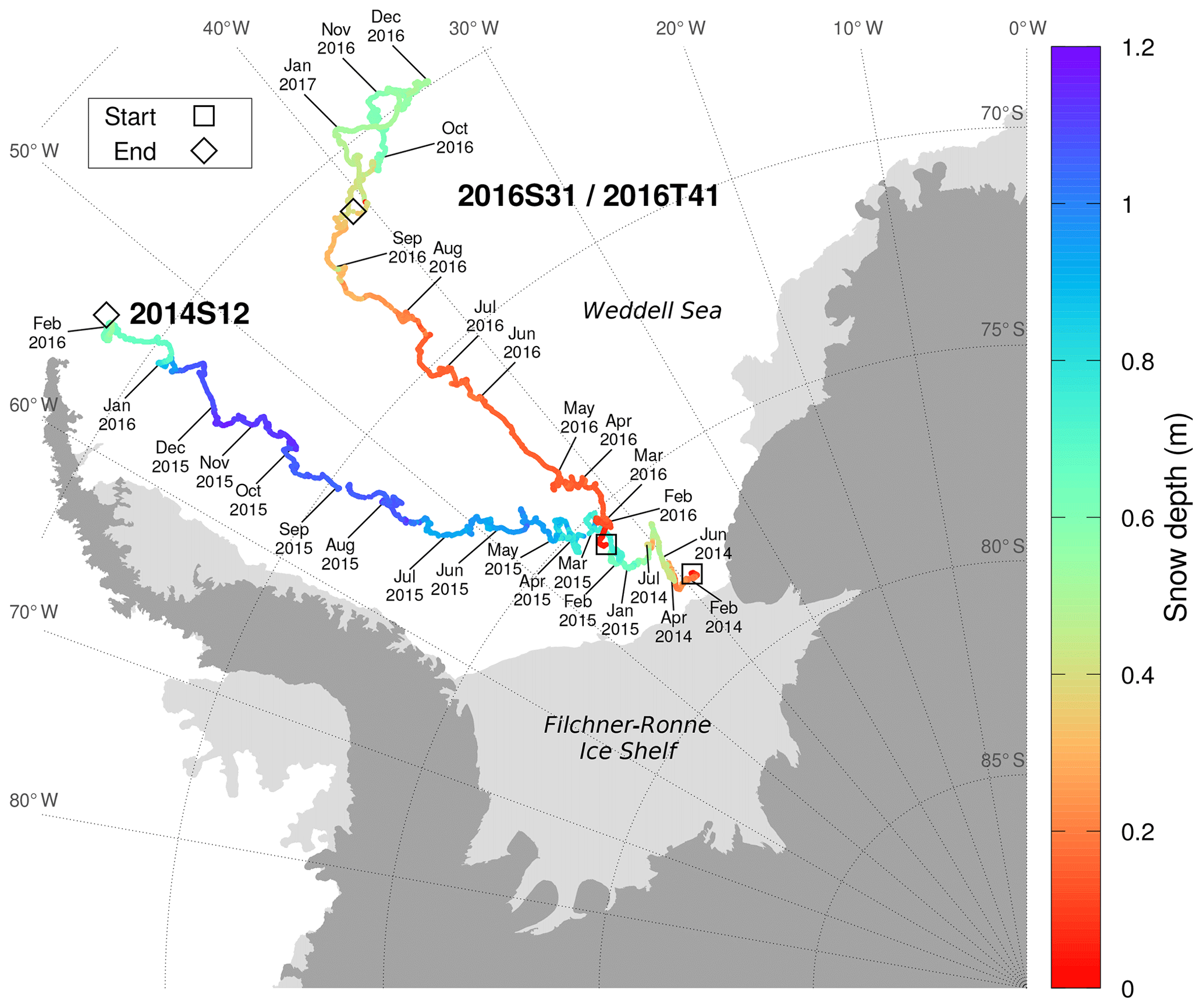
Figure 1Trajectories of the two snow buoys used for the simulations. The average snow depth measured by the four snow depth sensors from each snow buoy is shown in color. Labels show the position of the respective snow buoy on the first day of the month. For buoy 2014S12, some labels at the beginning have been omitted for readability. The deployment location (start) is denoted by a square; the location of the last received data from the buoy (end) is denoted by a diamond. The collocated IMB for the 2014S12 snow buoy (2014T9) stopped transmitting data shortly after installation and is ignored in the analysis. The collocated IMB to snow buoy 2016S31 is 2016T41.

In unsaturated conditions, the van Genuchten–Mualem model (Mualem, 1976) is used to relate the hydraulic conductivity in saturated conditions (Eqs. 22 and 23) to unsaturated conditions. For averaging the hydraulic conductivity between elements, we use the geometric mean (Wever et al., 2015), which is the preferred method (Haverkamp and Vauclin, 1979; Celia et al., 1990). Furthermore, in unsaturated conditions, the van Genuchten model is used for the water retention curve, which describes the relationship between capillary suction and LWC (van Genuchten, 1980). The coefficients in this parameterization of water retention in snow are based on the work by Yamaguchi et al. (2012). We extend this parameterization over the full porosity range, in absence of any information of water retention in sea ice as a function of salinity and LWC. It has a relatively small impact, as the largest part of the sea ice is below sea level and the model typically simulates saturated conditions here.

3.1 In situ buoys

We apply the sea ice version of SNOWPACK to snow and sea ice properties measured from two snow buoys (Nicolaus et al., 2017) and one ice mass-balance buoy (IMB) in the Weddell Sea, Antarctica. Snow buoys are autonomous ice-tethered instruments, which measure snow surface height changes with four ultrasonic sensors at approximately 1.5 m above the snow–ice interface. The four sensors were used to identify if the buoys remained stable on the ice. We construct a time series of the surface elevation referenced to the initial snow–ice interface upon installation of the buoy by averaging the four ultrasonic sensors. In addition to the surface elevation, the snow buoys measure barometric air pressure and air temperature.

Each IMB consists of a 4.8 m long thermistor chain, with a vertical sensor spacing of 0.02 m, and measures sea ice temperatures. From the measurements, interfaces between air, snow, sea ice, and sea water can be determined. The instruments are described by Jackson et al. (2013). It turned out to be good practice to co-deploy snow buoys and thermistor chain IMBs in order to observe snow depth and sea ice properties at the same time. The full data set of all these Lagrangian observations is available from http://www.meereisportal.de (last access: 14 June 2018) (Grosfeld et al., 2015).

The two selected snow buoys (snow buoys 2014S12, Nicolaus and Schwegmann, 2017, and 2016S31, Arndt et al., 2017) have long time series and cover different trajectories, as shown in Fig. 1. Unfortunately, IMB 2014T9 collocated with snow buoy 2014S12 stopped transmitting data soon after deployment. IMB 2016T41, collocated with snow buoy 2016S31 measured for almost the same period as the snow buoy. However, comparisons are limited to the sea ice temperature and ice thickness, excluding the snow cover on top, because the IMB was deployed directly onto the snow surface, without room to accommodate snow accumulations after installation. Thus, the thermistor chain does not measure the snow cover properties, except for the lowest few centimeters.

Figure 1 shows the trajectories with labels marking the location at the first of each month. Snow buoy 2014S12 was deployed on 17 January 2014 and remained in the same area very close to the Filchner–Ronne Ice Shelf for the first year. From February 2015 onward, the snow buoy drifted northward parallel to the Antarctic Peninsula until data transmission was lost on 1 February 2016. During the last 18 h no valid snow depth data were transmitted and the drift speeds were relatively high, suggesting that it is not a transmission or data logger failure but rather an indication that flow deformation or breakup is the likely cause of the loss of the snow buoy. We consider this particular snow buoy due to its long time span, even though a collocated IMB data set is not available.

Snow buoy 2016S31, collocated with IMB 2016T41, was deployed on 16 January 2016. This deployment first drifted on a predominantly northward course. Around 1 December, the northernmost position was reached and the deployment drifted southward again. The snow buoy transmitted data until 15 January 2017, 02:00 UTC, shortly before the last data transmission by the IMB (5 February 2017, 07:13 UTC). This combination of snow buoy and IMB is interesting for the long time span of collocated measurements.

3.2 Initial conditions

To start each simulation, a description of the initial sea ice state is required. Upon installation of each snow buoy, the ice thickness, snow thickness, and freeboard were determined. For simulations of these snow buoys, we distinguish three categories: (i) sea ice below sea level (ice thickness minus freeboard), (ii) sea ice above sea level (freeboard), and (iii) snow.

For the part of the sea ice below sea level, the volumetric ice content θ_i was fixed to 0.95, and the volumetric water content θ_w was subsequently calculated as

This formulation leaves a small volumetric air content which can be filled when water refreezes and thereby expands. This is currently required for the stability of the numerical schemes in the SNOWPACK model, but in reality refreezing water would increase the pressure in the brine. The element temperature was initialized by the value recorded by the IMB upon installation. As it takes time for the thermistor chain to freeze into the ice and adapt to the surrounding ice temperature, this temperature is mostly representative of the ocean water. The brine salinity was set as the salinity for which the melting point corresponds to the measured temperatures.

For the part of sea ice above sea level, the volumetric ice content θ_i was also fixed to 0.95, but the remaining space was assigned to air content and the bulk salinity was set to 0 g kg⁻¹. In field studies, it was found that brine may exist above sea level, due to capillary wicking, or brine content is retained because of low conductivity in the brine channels (e.g., Cox and Weeks, 1974; Massom et al., 2001).

The initial snow layer was 10 cm for snow buoy 2014S12 and 2 cm for 2016S31. The snow cover was initialized with a density of 275 kg m⁻³ and a grain size of 0.15 mm. The grain shape was initialized as depth hoar with a sphericity and dendricity of 0. As the majority of the snowpack builds during the model simulations, the simulations are rather insensitive to the choice of initial snowpack properties. The element temperature was derived from the thermistor chain measurements. Finally, the depth of each element was set to 0.02 m.

3.3 Forcing data

Simulations with the SNOWPACK model require air temperature, relative humidity, incoming shortwave radiation, incoming longwave radiation, wind speed, and precipitation. Here, we used the European Centre for Medium-range Weather Forecasts ECMFW Reanalysis 5 (ERA5, ERA, 2017) data to provide these parameters to drive the simulations. For each time step and location, the simulated weather at the closest grid point in the ERA5 model was taken.

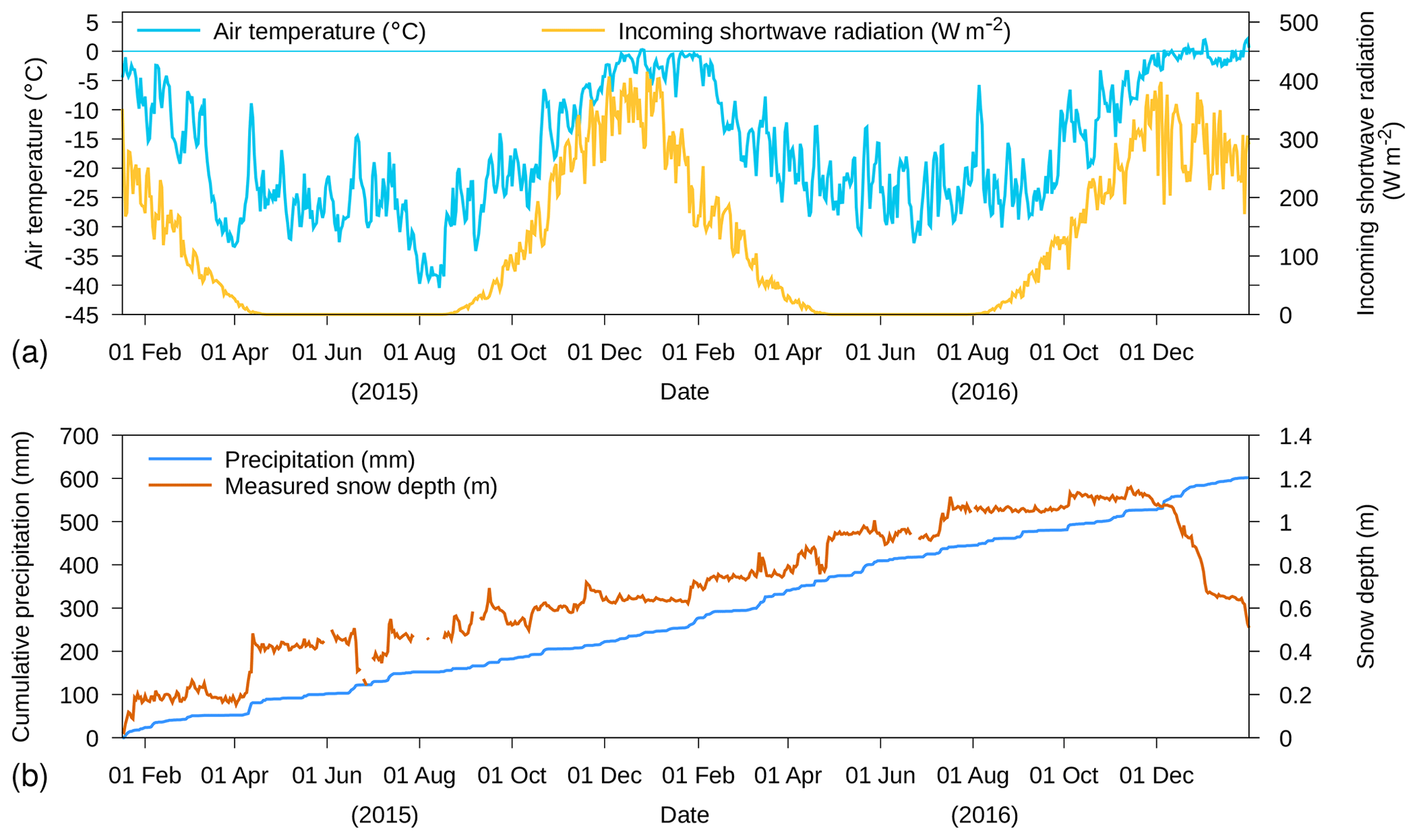
Figure 2Meteorological forcing data from ERA5 for snow buoy 2014S12 for (a) daily average air temperature and daily average incoming shortwave radiation and (b) cumulative precipitation. In (b), measured snow depth by the buoy is also shown.

Download

Figure 2 shows the daily average air temperature, incoming shortwave radiation, and cumulative precipitation from the ERA5 forcing for snow buoy 2014S12. Additionally, the measured snow depth by the buoy is shown. We find that the daily average air temperature was mostly below 0 ^∘C, reaching −40 ^∘C in 2015. Near the end of the time series, when the snow buoy stopped transmitting data, daily average air temperature varied around 0 ^∘C. It can be expected that positive temperatures during midday are associated with enhanced snowmelt, which is indicated by the rapid decrease in measured snow depth starting from December 2016 onward. During austral winter 2015 and 2016, the snow buoy was located below the polar circle and consequently, there was no incoming shortwave radiation. In austral summer 2016/2017, the snow buoy drifted above the polar circle. Nevertheless, the average incoming shortwave radiation in the first austral summer is similar to the second austral summer. The cumulative precipitation from ERA5 reached around 600 mm for the almost 2 years that the buoy was operative. The buoy recorded 1.2 m of snow accumulation. A marked increase in snow depth around 1 April 2015 is accompanied by only a relatively small precipitation event. Except for this event, both the snow depth as well as the cumulative precipitation show a gradual increase over the 2 years until the melt phase starts.

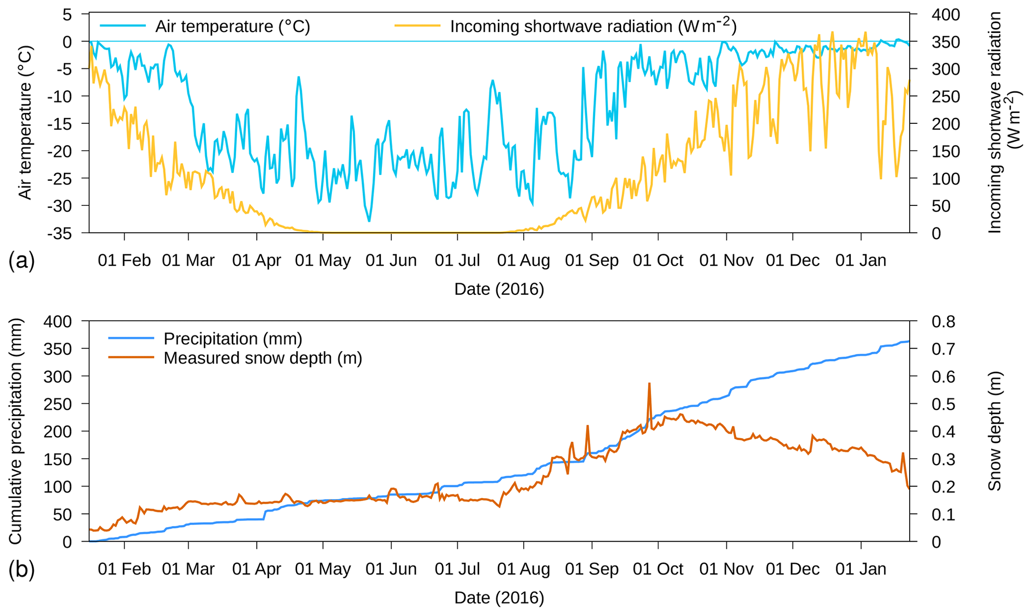
Figure 3Meteorological forcing data from ERA5 for snow buoy 2016S31 for (a) daily average air temperature and daily average incoming shortwave radiation and (b) cumulative precipitation. In (b), measured snow depth by the buoy is also shown.

Download

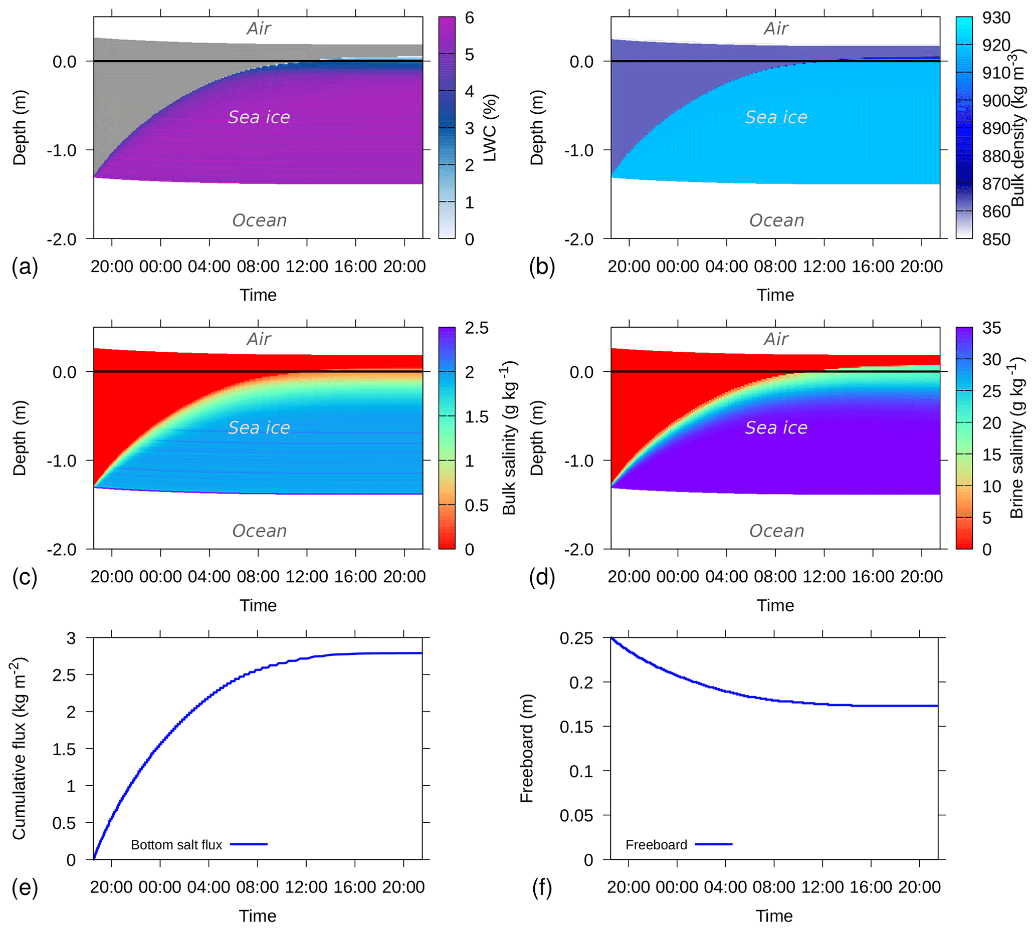
Figure 4Example simulation where initially dry, porous freshwater ice with 94% volumetric ice content is placed into ocean water with a salinity of 35 g kg⁻¹. Shown are (a) liquid water content (LWC), (b) bulk density, (c) bulk salinity, (d) brine salinity, (e) cumulative salt flux at the bottom of the sea ice, and (f) freeboard. In (a), dry parts of the ice are colored grey. In (a–d), the depth on the y axis is relative to sea level, i.e., sea level is 0 and indicated by the solid black line.

Download

Figure 3 shows the daily average air temperature, incoming shortwave radiation and cumulative precipitation from the ERA5 forcing for snow buoy 2016S31. The yearly cycle in air temperature is similar to the year 2016 for snow buoy 2014S12, with daily air temperatures reaching around −30 ^∘C in austral winter. In austral summer, daily average air temperatures around 0 ^∘C suggest melting conditions, particularly from November 2016 to January 2017. This is reflected by the decrease in measured snow depth for this period. The snow buoy was also located south of the polar circle, resulting in the absence of shortwave radiation during austral winter. The precipitation sum for the year that the snow buoy was operative amounted to 350 mm. The snow depth does not change between March and July 2016 and shows an increase between August and October, after which a decrease occurs. The cumulative precipitation shows a similar pattern, with low precipitation between March and July, followed by a steady increase afterwards. Only during the melt phase is the increase in cumulative precipitation not reflected by an increase in snow depth.

SNOWPACK has the possibility to either use a precipitation time series as input to determine when snow fall occurs or to use a time series of snow depth to interpret increases in measured snow depth as snow fall events when simulated snow depth is less than the measured snow depth (Lehning et al., 1999). Note that there is no downward correction when the measured snow depth is below the simulated snow depth (in the case of underestimated melt, surface sublimation or settling, or snow erosion by wind, etc.). In order to use the snow-depth-driven method for the snow buoys and base the mass balance on snow buoy data, a layer can be marked in the simulations and tracked throughout the snow–sea-ice continuum. By marking the layer that corresponds to the reference level for the snow depth measurements, the measured snow depth can be tracked relative to this marked layer. The output routines of the model have been adapted accordingly to reference the output to either the sea level or to the marked reference layer.

The ocean heat flux determines the ice mass balance at the bottom of the ice. Its value can be highly variable and dependent on ocean conditions below the sea ice (Ackley et al., 2015). From that study, we use a value of 8 W m⁻², unless otherwise noted.

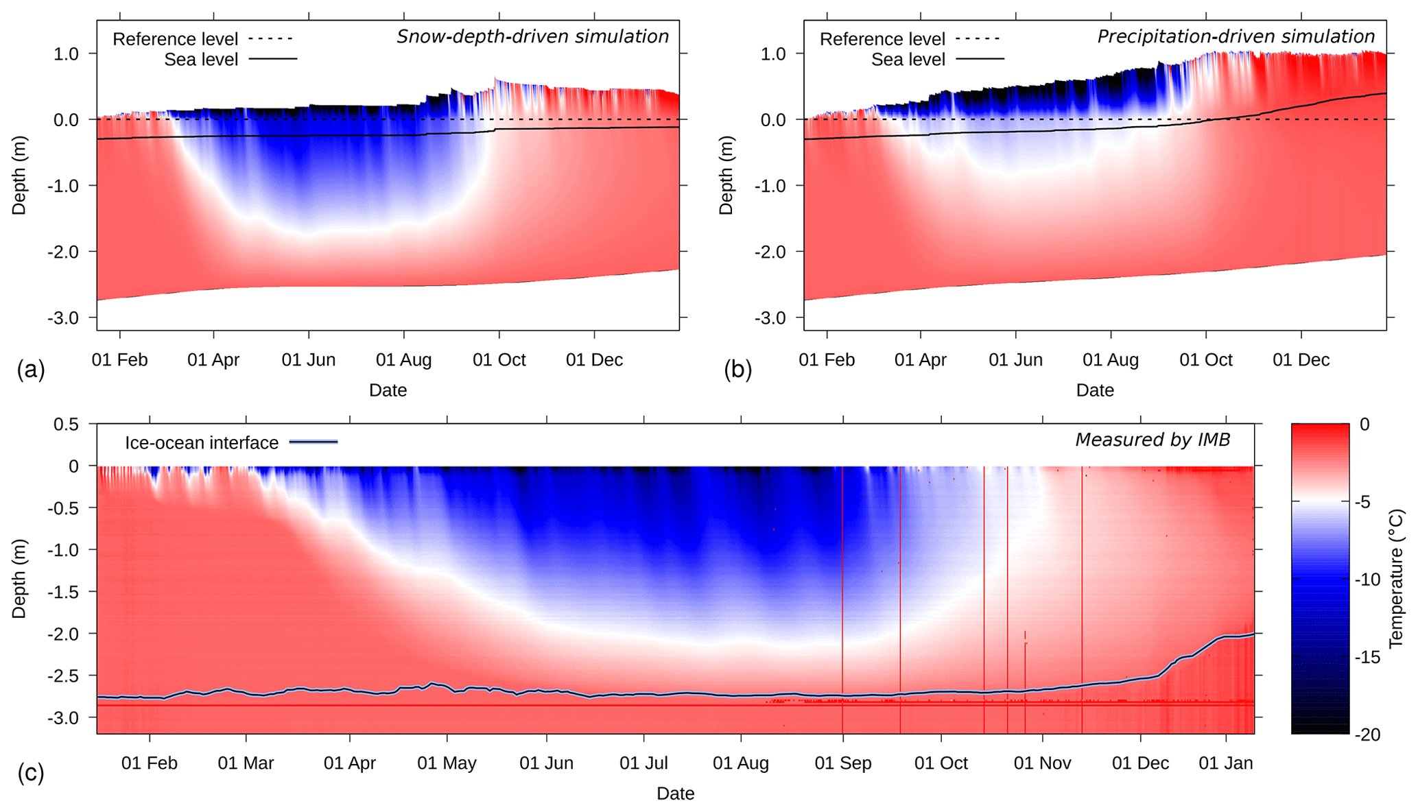
Figure 5Snow and ice temperatures for snow buoy 2016S31/IMB 2016T41, for (a) simulations driven by in situ measured snow depth, (b) simulations driven by ERA5 precipitation, and (c) measured temperatures by the IMB. The depth on the y axis is defined relative to the snow–ice interface, as determined upon installation (dashed line). In (a) and (b), the solid line denotes the sea level as determined by the simulations. In (c), the blue/black line denotes the ocean–ice interface, as determined from the IMB measurements.

Download

4.1 Example simulation

Figure 4 shows an example of model behavior when an initially dry and fresh ice layer with a thickness of 1.58 m, consisting of 94 % ice and 6 % air expressed as volumetric content, is positioned in ocean water with a salinity of 35 g kg⁻¹. The positive pressure head at the bottom of the sea ice corresponds with the pressure exerted by the displaced water. As a consequence, saline water enters the ice matrix (Fig. 4a, c), until it is in equilibrium with the sea level. The initial rate follows the saturated hydraulic conductivity for sea ice with a pore space of 6 %, which is $\mathrm{3.55}\times {\mathrm{10}}^{-\mathrm{5}}$ m s⁻¹ (Eq. 23).

As the pressure difference of the liquid water inside the ice matrix and the surrounding ocean water is decreasing, the salt influx rate decreases over time (Fig. 4e). The brine salinity corresponds to the salinity of ocean water (35 g kg⁻¹, see Fig. 4d), corresponding to a bulk salinity of 1.65 g kg⁻¹ (see Fig. 4c). The added mass to the sea ice (Fig. 4b) causes the ice to sink deeper inside the ocean water, decreasing the freeboard (Fig. 4f).

This example illustrates that the Crank–Nicolson scheme does not preserve the sharp transition in salinity, as both the bulk (Fig. 4c) as well as the brine (Fig. 4d) salinity shows smoothing behavior at the saline water front. This reduces the pore space by refreezing to maintain thermal equilibrium, reducing the saturated hydraulic conductivity in the wetting front region.

4.2 Temperature validation

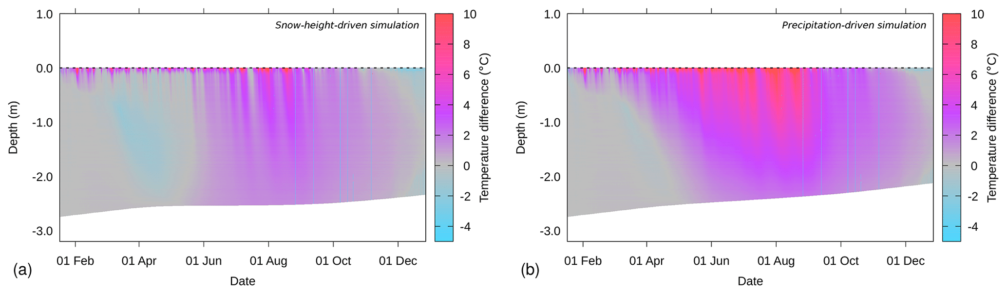
Figure 6Difference between simulated and measured snow and ice temperatures for snow buoy 2016S31/IMB 2016T41, for (a) simulations driven by in situ measured snow depth and (b) simulations driven by ERA5 precipitation. The depth on the y axis is defined relative to the snow–ice interface, as determined upon installation.

Download

Figure 5a and b show the simulated temperature of the snow–sea-ice system for simulations driven by in situ measured snow depth and ERA5 precipitation, respectively. Dashed lines denote the reference level, i.e., the snow–ice interface as determined upon installation of the snow buoy. The sea level as calculated from hydrostatic balance is indicated by the solid line. For the snow-depth-driven simulations, the sea level stays below the snow–ice interface, indicating that freeboard is positive during the whole simulation period. However, for the precipitation-driven simulations, there is more snowfall, which causes negative freeboard from October onward.

Figure 5c shows the measured sea ice temperatures from the corresponding IMB. Note that for this IMB, the thermistor chain does not extend above the initial 2 cm snow layer on top of the sea ice, such that the time evolution of the snow cover is not recorded by the IMB. We find that the IMB confirms the strong cooling of the sea ice during the austral winter months, as found in the simulations, as well as the near-surface warming to the melting point of freshwater shortly before the last transmission by the buoy.

Figure 6 shows difference plots of measured and simulated ice temperatures. Figure 6a compares the snow-depth-driven simulations (i.e., Fig. 5a minus Fig. 5c) and Fig. 6b compares the precipitation-driven simulations (i.e., Fig. 5b minus Fig. 5c). Positive values denote an overestimated temperature by the model and vice versa. Note that the bottom of the sea ice in the simulations is typically above the ice–ocean interface in the IMB data.

The comparison shows that in the period March to May, the snow-depth-driven simulation slightly underestimates the sea ice temperatures, which suggests an overestimation of the initial cooling of the sea ice towards austral winter. Both simulations overestimate the lowest temperatures reached in winter by up to 6–15 ^∘C near the snow–ice interface, which is located at the top of the thermistor chain. Similarly, incidental cooling in near-surface sea ice layers in February and March is also underestimated. This could on the one hand indicate an overestimation of incoming energy or an underestimation of outgoing energy in the forcing data or by the model. On the other hand, new snow density in polar regions is higher than in alpine snow covers, due to the impact of drifting snow (Groot Zwaaftink et al., 2013; Steger et al., 2017). Even though the new snow density in SNOWPACK is parameterized using wind speed (in addition to air temperature, surface temperature, and relative humidity), and also the snow settling formulation employed here leads to higher densities under the influence of wind (Lehning et al., 2002b), near-surface (new) snow density is likely still underestimated. An underestimated (new) snow density would result in an underestimated thermal conductivity and overestimated thermal insulation in the model, as thermal conductivity typically increases with increasing snow density. Heat from the sea ice part would then not be able to be sufficiently transported through the snowpack and exchanged with the atmosphere.

The simulations driven by ERA5 precipitation show about twice as much snow accumulating on the sea ice (Fig. 5b) compared to accumulations determined from the snow height measurements (Fig. 5a). Also the reanalysis provides precipitation (and thus snow accumulating) in the austral winter time, which is not found in the snow depth time series. This is not necessarily a bias in ERA5, because snow erosion by wind can keep the snow depth constant over extended periods of time. Furthermore, if new snow density is underestimated, snow depth is likely overestimated, even though snow settling reduces the discrepancy. Due to these factors, the total snow depth may be overestimated by the ERA5 input at the end of the simulation. Furthermore, the thick snow cover in the precipitation-driven simulation better insulates the underlying ice, resulting in a stronger overestimation of ice temperatures compared to the snow-height-driven simulation.

The thermistor chain is also used to determine the heat capacity by heating the chain for 1 or 2 min and analyzing the temperature response. By combining the absolute temperatures and the heating rates, the ice–ocean interface has been manually determined and is shown in Fig. 5c. The IMB data confirm the modeling result that the strong negative energy balance at the top of the snow–sea-ice system during austral winter has not resulted in an ice thickness increase. The warmer sea ice in the precipitation-driven simulations resulted in a thinning of the ice by the ocean heat flux, which is not confirmed by the IMB data. The decrease in ice thickness in December 2016 is not reproduced by either one of the simulation setups. The trajectory of the buoy shows a marked change in drift direction (Fig. 1), changing from a northward to a southward drifting course during this period. This change of direction may have been accompanied by an intrusion of warm ocean water below the sea ice and an increased ocean heat flux.

LWC, bulk and brine salinity, as well as the bottom salt flux for the simulations driven by measured snow depth are shown in Fig. 7. LWC (Fig. 7a) shows a strong reduction in austral winter due to the freezing brine, causing brine salinity to increase (Fig. 7c). The snow is dry most of the time, except towards the end of the simulation when meltwater percolates downward. Furthermore, we find a thin layer with low values of LWC just above sea level. This is caused by capillary forces causing upward motion of sea water above sea level.

Figure 7b shows that the bulk salinity of the sea ice hardly changes over the course of the simulation, whereas the brine salinity (Fig. 7c) clearly shows a relationship with the temperature. This reflects the prescribed thermal equilibrium between brine and the ice, assuming that the brine is at melting temperature. Figure 7d shows that the added weight of the accumulating snow pushes the sea ice deeper into the ocean, increasing the pressure head at the bottom of the sea ice. This leads to an influx of saline water, even though the sea level remains below the snow–ice interface. Combined with rising temperatures, a thin layer with increased bulk salinity and increased LWC forms around and just below sea level around 1 October.

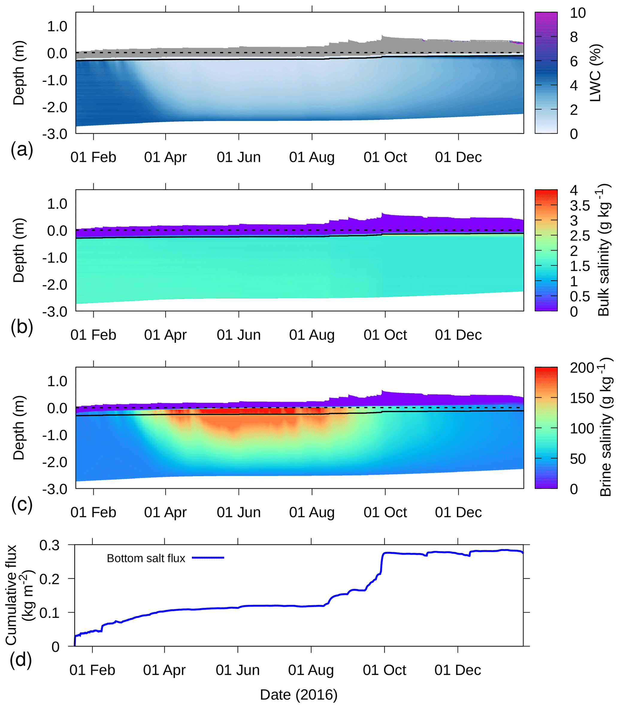
Figure 7Example simulation for snow buoy 2016S31, where measured snow depth was used to derive the precipitation events, for (a) LWC, (b) bulk salinity, (c) brine salinity, and (d) cumulative salt flux at the bottom of the sea ice. In (a), dry parts of the snow–sea-ice system are colored grey. In (a–c), the depth is defined relative to the snow–ice interface, as determined upon installation (dashed line). The solid line denotes the sea level as determined by the simulation. In (d), an increasing cumulative flux denotes inflow and vice versa.

Download

Figure 8Example simulation for buoy 2014S12, where measured snow depth was used to derive the precipitation events, for (a) temperature, (b) LWC, (c) bulk salinity, (d) brine salinity, and (e) cumulative salt flux at the bottom of the sea ice. In (b), dry parts of the snow–sea-ice system are colored grey. In (a–d), the depth is defined relative to the snow–ice interface, as determined upon installation (dashed line). The solid line denotes the sea level as determined by the simulation. In (e), an increasing cumulative flux denotes inflow and vice versa.

Download

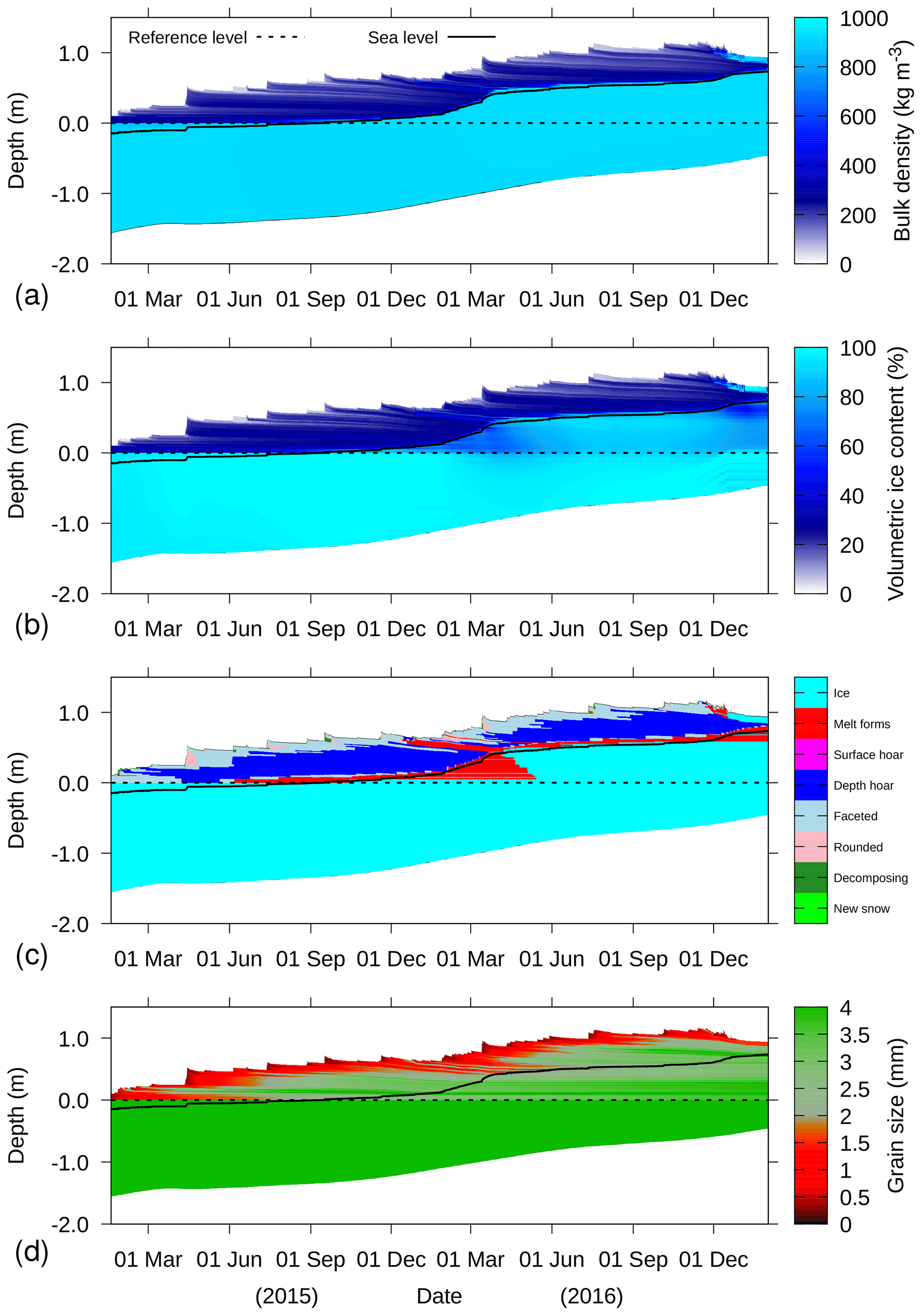
Figure 9Example simulation for buoy 2014S12, where measured snow depth was used to derive the precipitation events, for (a) total bulk density, (b) volumetric ice content, (c) grain type, and (d) grain size. The depth on the y axis is defined relative to the snow–ice interface, as determined upon installation (dashed line). The solid line denotes the sea level as determined by the simulation.

Download

4.3 Flooding and superimposed ice formation

Figures 8 and 9 show an example simulation for snow buoy 2014S12. The simulations were driven by the snow depth measurements from the buoy. Upon installation of the buoy, the snow depth was referenced to the sea ice surface. This reference level is shown by the dashed line. Due to basal ice melt and growth, as well as additional snowfall, the simulated sea level became higher with regard to the snow depth sensor, as indicated by the solid line. This is congruent with a negative freeboard. It indicates that significant flooding occurred, as also evidenced by the LWC in Fig. 8b and associated high-bulk salinity (Fig. 8c). Figure 9a shows that the bulk density of the flooded part is similar to the underlying ice density, illustrating the depletion of pore space. Figure 9b shows an increase in ice content in the flooded layers, indicating that a substantial amount of the sea water flooding the snow refroze, adding considerable ice mass.

The simulated temperature (Fig. 8a) shows the two austral winters with low temperatures, and the two austral summers with temperatures close to 0 ^∘C. Interestingly, the low temperatures in the first austral winter impacted the part below sea level stronger than the second austral winter, as demonstrated by the lower temperatures in that part of the domain. During the second austral winter, flooding in the simulation increased the liquid water content of the snow, and consequently, much of the energy loss by the sea ice in this period was balanced by the energy release from refreezing liquid water, rather than decreasing temperatures.

Figure 8e shows that flooding also leads to a strong influx of salt to the snow-sea ice system. The flooding saturates the snow, which has significant pore space compared to the sea ice. Therefore, snowfall events of similar magnitude have different effects on the salt influx, depending on whether or not flooding occurs at the time.

Note that the flooding, as depicted in simulations with the Richards equation coupled to the transport equation, is governed by the hydraulic conductivity of ice. In cold ice, hydraulic conductivity can be so low that negative freeboard remains for extended period of times, even without flooding. On the other hand, flooding may also be triggered by deformation and cracking of the sea ice, combined with lateral flow effects. However, Maksym and Jeffries (2000) have shown that the simpler assumption (i.e., negative freeboard will trigger flooding) can already yield satisfying results. In the model, the maximum ice content is fixed to 0.99 m³ m⁻³ and is typically lower, such that hydraulic conductivity is generally large enough for instantaneous flooding.

The brine salinity in Fig. 8d shows spurious oscillations. These originate from the lower boundary and could be caused by the strong transition of brine salinity to ocean salinity. Also, the oscillations are partly attributed to the maximum allowed ice content of 99 % in the simulations, as they occur in the same area. The exact numerical mechanism and a possible solution are currently unknown.

Figure 9c and d show the snow microstructure as simulated by the model. Even though validation for this specific floe is not possible, we find several features consistent with other field observations. For example, a wet slush layer (coloured red) at the interface between snow and ice is visible, triggered by capillary suction and flooding. This is also reported in Nicolaus et al. (2009) and Arndt and Paul (2018) for the same geographical region. Even though those field observations report the presence of depth hoar layers in snowpacks, particularly in deeper snowpacks (exceeding 30 cm), the simulations seem to show deeper depth hoar layers (coloured blue) than reported in field observations. The field observations often report wind slabs or other hard layers in between depth hoar layers. Simulating those kind of layers is a well-known problem for snowpack models (Domine et al., 2019).

The grain size shown in Fig. 9d ranges from 2 to 2.5 mm in the depth hoar layers at the base of the snowpack to 0.5–1 mm near the top of the snowpack. These simulated grain sizes corresponds to the range of values reported by the field studies listed earlier (1–5 mm), yet exact validation remains difficult.

4.4 Forced warming and cooling

Warming conditions increase the brine volume and the hydraulic conductivity of the sea ice but can also cause freshwater percolation from snowmelt. Similarly, cooling conditions decrease brine volume and increase brine salinity and density. When brine channels allow, the dense brine may drain from the sea ice.

To test how the model reacts to continuous warming or cooling conditions, we used snow buoy 2016S31 for two experiments where we forced constant warming and constant cooling conditions by modifying the meteorological driving data starting 1 April 2016. To force warming conditions, we prescribed a constant air temperature of +5 ^∘C, a relative humidity of 80 %, a wind speed of 3 m s⁻¹, and an incoming shortwave radiation of 300 W m⁻².

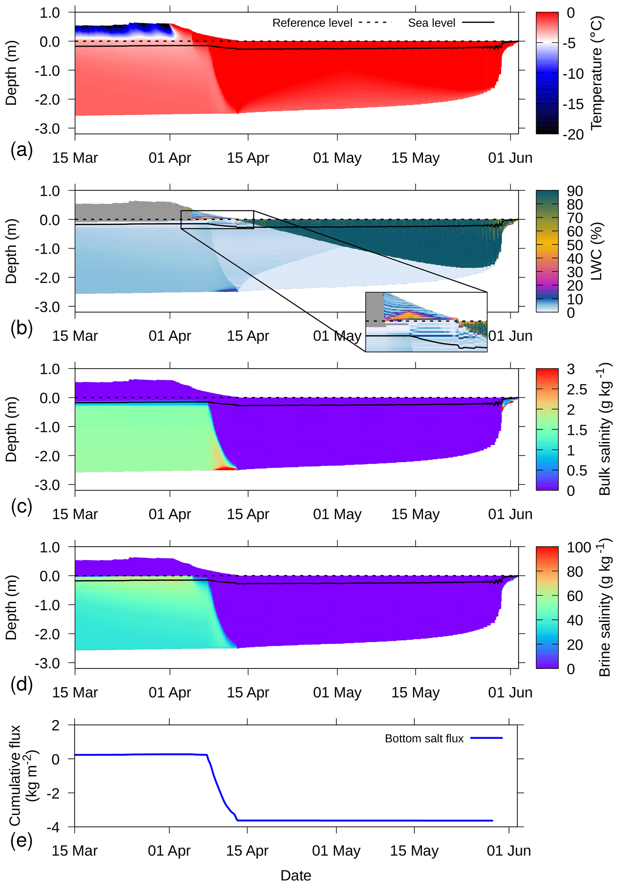
Figure 10Simulation for 2016S31, where from 1 April onward, melting conditions were enforced, for (a) temperature, (b) LWC, (c) bulk salinity, (d) brine salinity, and (e) cumulative salt flux at the bottom of the sea ice. In (b), dry parts of the snow–sea-ice system are colored grey and an inset shows the water percolating through the snow and ponding on the snow–ice interface. In (a–d), the depth on the y axis is defined relative to the snow–ice interface, as determined upon installation (dashed line). The solid line denotes the sea level as determined by the simulations. An increasing cumulative flux denotes inflow and vice versa.

Download

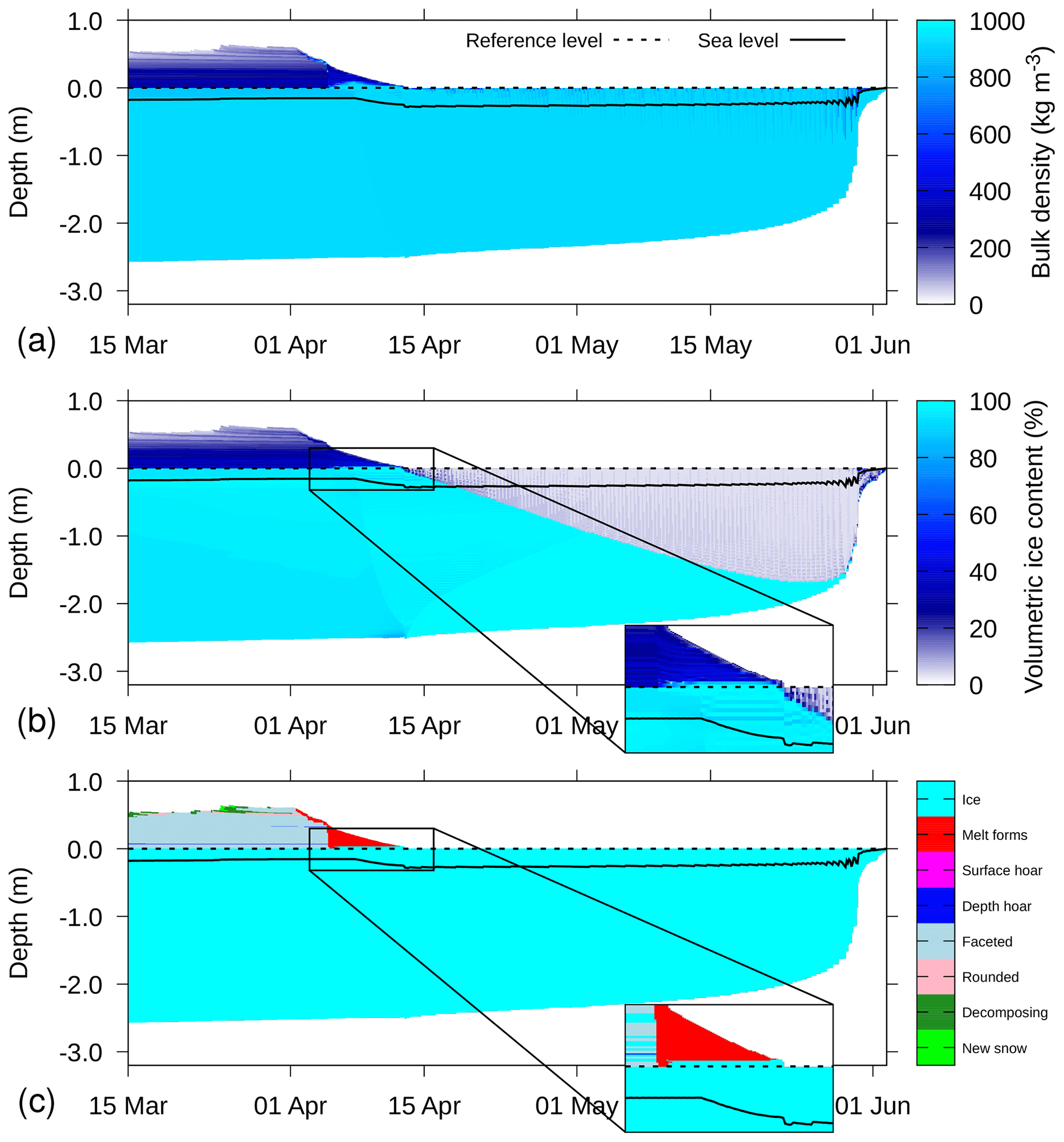
Figure 11Simulation for 2016S31, where from 1 April onward, melting conditions were enforced, for (a) total bulk density, (b) volumetric ice content, and (c) grain type. In (b) and (c), an inset shows the superimposed ice formation on the snow–ice interface. The depth on the y axis is defined relative to the snow–ice interface, as determined upon installation (dashed line). The solid line denotes the sea level as determined by the simulations.

Download

Figures 10 and 11 show the simulation result for the warming experiment. Figure 10 shows that as soon as melting conditions were enforced (starting 1 April), the snowpack very quickly reached melting temperature. The freshwater percolating as a result from snowmelt first started accumulating on below-freezing sea ice with low porosity (see Fig. 10b). This process is visible in April and leads to a thin layer of superimposed ice (Fig. 11b and c). Starting 15 April, the bulk density of the snow–sea-ice system was homogeneously around ice density, showing that the pore space has been depleted (Fig. 11a).

The freshwater started flushing the ice around 10 April, leading to a rapid reduction in bulk and brine salinity (Fig. 10c, d), due to the outflow of saline water at the bottom of the sea ice (Fig. 10e). When the brine salinity decreases, water freezes and the permeability of the sea ice is low compared to the surface melt. We find that meltwater accumulates on the top of the sea ice (Fig. 10b), which can be interpreted as the formation of a melt pond.

The sea ice thins continuously upon continued warming (Fig. 11b), until the ice has melted and the melt pond disappears. At this point, the simulations showed strong instabilities in the bottom salt flux, such that the cumulative flux in Fig. 10e is only shown for the time period with ice below the liquid water. Note that the melt pond in the model consists of a little bit of ice (Fig. 11b), which results from the SNOWPACK numerics.

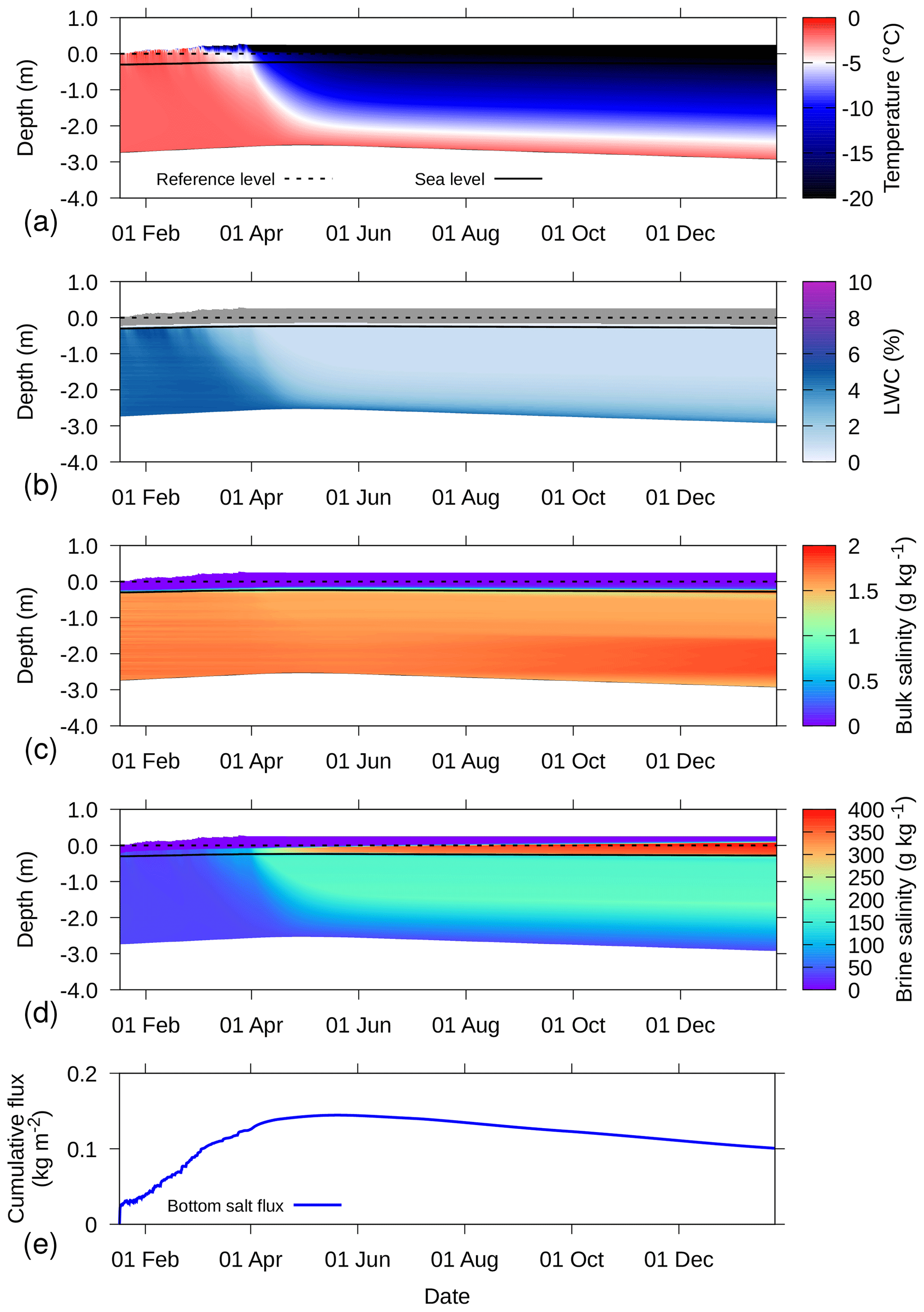
Figure 12Simulation for 2016S31, where from 1 April onward, cooling conditions are enforced, for (a) temperature, (b) LWC, (c) bulk salinity, (d) brine salinity, and (e) cumulative salt flux at the bottom of the sea ice. In (b), dry parts of the snow–sea-ice system are colored grey. In (a–d), the depth on the y axis is defined relative to the snow–ice interface, as determined upon installation (dashed line). The solid line denotes the sea level as determined by the simulations. An increasing cumulative flux denotes inflow and vice versa.

Download

Figure 12 shows an example where cooling conditions were enforced. Similar to the warming example, the meteorological forcing conditions were replaced from 1 April onward by setting a constant air temperature of −30 ^∘C, a wind speed of 1 m s⁻¹, and no incoming shortwave radiation. The ocean heat flux was set at 8 W m⁻². As soon as cooling conditions were present, a freezing front progressed through the sea ice. The interface between the sea ice and the ocean remained at the freezing point of ocean water, while the sea ice froze and increased thickness.

With the decrease in temperature, brine salinity increased (Fig. 12d). This is achieved by freezing the liquid water, as shown by the decrease in LWC (Fig. 12b). An increase in brine salinity also increases the density of the brine. This may lead to flushing of the sea ice, when the heavy brine moves downward and is replaced by lighter ocean water. However, in our simulations, there is only a very small outflow of salinity at the bottom (Fig. 12e) and the bulk salinity remains approximately constant (Fig. 12c). This result shows that without a description of the convective processes in sea ice resulting from cooling (Griewank and Notz, 2013), the salinity depletion found due to cooling is strongly underestimated by this model approach.

4.5 Thin ice

A final test is run by starting with only 2 cm of ice and constant atmospheric conditions to simulate thin ice evolution. The atmospheric conditions were set to −10 ^∘C air temperature, 100 % relative humidity, no wind speed, no incoming solar radiation, and a constant incoming longwave radiation of 230 W m⁻². The ocean heat flux was set to 0 W m⁻².

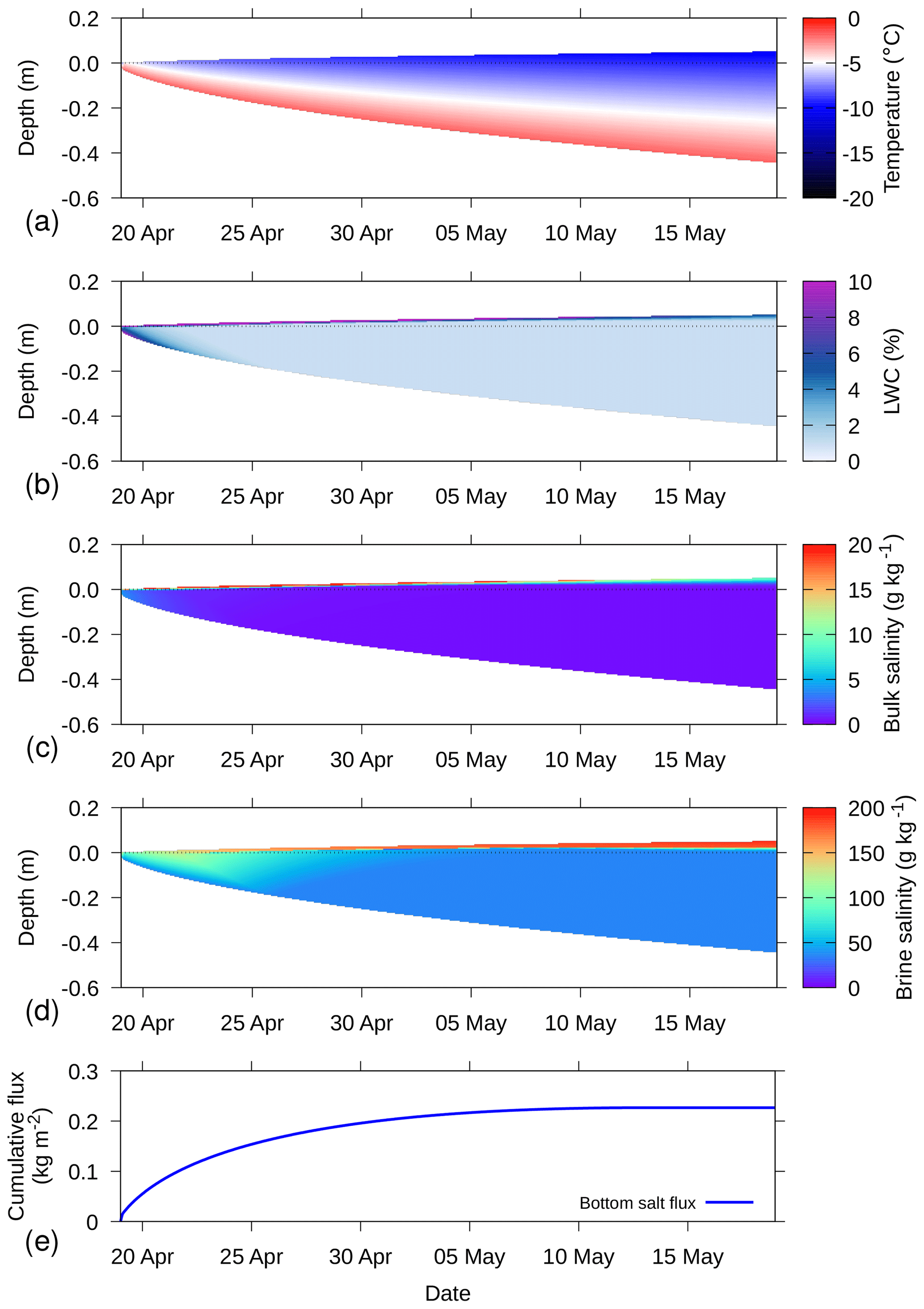
Figure 13Simulation for ice growth of thin ice, for (a) temperature, (b) LWC, (c) bulk salinity, (d) brine salinity, and (e) cumulative salt flux at the bottom of the sea ice. In (a–d), the depth on the y axis is defined relative to sea level. An increasing cumulative flux denotes inflow and vice versa.

Download

The simulations were run for 1 month, which resulted in approximately 50 cm ice growth (Fig. 13). The temperature distribution (Fig. 13a) shows a very strong gradient, as the bottom temperature is forced to the ocean water temperature, whereas the surface cools from radiation loss and sensible and latent heat exchange. The relatively warm sea ice compared to the air temperature results in a latent heat flux directed to the atmosphere, even though relative humidity is 100 %. The evaporation at the top of the sea ice leads to an outflow of freshwater at the top of the snowpack, resulting in an accumulation of salt near the surface (e.g., Kaleschke et al., 2004; Domine et al., 2005). This is found in Fig. 13b and c in a salty slush layer at the surface with high LWC and high-bulk salinity. The brine salinity (Fig. 13d) mimics the temperature distribution (Fig. 13a) because of the forced thermal equilibrium with the brine by the model. When the ice is very thin, the evaporation at the top of the ice causes an influx of salt at the bottom (Fig. 13e). The transport of salt from below decreases with increasing ice thickness, as capillary forces are not strong enough anymore to bridge the freeboard.